A parallel implementation on modern hardware for geo electrical tomographical software

cudaHostAlloc which allows host memory to be into CUDA address space providing asynchronous transparent access to data without explicit copy using cudaMemcpy.

A notable property that applications using CUDA have is the memory sharing between CUDA memory and OpenGL or DirectX memory. This makes it quite convenient for scientific simulations that can push computed results on GPU shaders directly to the display device by calling appropriate APIs. This feature is also useful in games and other graphic tasks.

Further information about CUDA programming can be found in the Nvidia CUDA Programming Guide [8].

1.2.3 Heterogeneous programming and OpenCL

The next platform is OpenCL (Open Computing Language) [24]. It was proposed by Apple and has now become a standard maintained by the Khronos group just like OpenGL. The first version of OpenCL came out in December 2008. OpenCL shares many similarities with CUDA but support heterogeneous computing on a wide range of platforms, including Intel and AMD CPUs; Nvidia and ATI GPUs; Cell processors, FPGAs, digital signal processors and other platforms. At the time of this writing, there are OpenCL implementations on most major parallel platforms although features and performance still varies.

OpenCL has a lowerlevel interface than CUDA, like the CUDA driver API. Programmers still write compute kernels but have to load them into the device command queue. This also makes OpenCL more flexible than CUDA as it can support both task parallelism and data parallelism. Data movements between the host and compute devices, as well as OpenCL tasks, are coordinated via command queues. Command queues provide a general way of specifying relationships between tasks, ensuring that tasks are executed in an order that satisfies the natural dependences in the computation. The OpenCL runtime is free to execute tasks in parallel if their

dependencies are satisfied, which provides a generalpurpose task parallel execution model. Tasks themselves can be comprised of dataparallel kernels, which apply a single function over a range of data elements, in parallel, allowing only restricted synchronization and communication during the execution of a kernel.

OpenCL’s data parallelism is quite like CUDA. There are many similar concepts to CUDA but with different names. Instead of grid and blocks, the kernel is executed over a similar index space with equal workgroups. The memory hierarchy also share many similarities with CUDA.

Có thể bạn quan tâm!

Xem toàn bộ 65 trang tài liệu này.

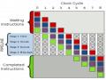
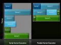
While the division of a kernel into workitems and workgroups supports data parallelism, task parallelism is supported via the command queue. Different kernels representing different tasks may be enqueued. Dependency between tasks can also be specified. Multiple command queues can also be created.

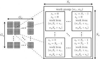
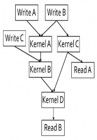
Figure 15 OpenCL data parallelism and task parallelism

Below is an example OpenCL code in the Nvidia GPU Computing SDK for computing dot product:

kernel void DotProduct (global float* a,global float* b,global float* c, int iNumElements)

{

// find position in global arrays int iGID = get_global_id(0);

// bound check (equivalent to the limit on a 'for' loop for standard/serial C code

if (iGID >= iNumElements)

{

return;

}

// process

int iInOffset = iGID << 2;

c[iGID] = a[iInOffset] * b[iInOffset]

+ a[iInOffset + 1] * b[iInOffset + 1]

+ a[iInOffset + 2] * b[iInOffset + 2]

+ a[iInOffset + 3] * b[iInOffset + 3];

}

Compared to CUDA, OpenCL has both task parallelism and data parallelism

while CUDA has limited support for task parallelism. However, this makes the OpenCL have a steeper learning curve. Writing portable OpenCL code with good performance on all architectures is still hard as there are many differences which call for platform specific optimizations. For example, while Nvidia hardware encourages the use of scalar code, AMD GPUs is designed for vector types such as float4 to get good performance. The efficiency of OpenCL model on CPUs versus CPUonly technologies such as OpenMP or TBB is a problem that needs further experiment. OpenCL drivers and support tools are also not as mature as established technologies. Support libraries is also a factor worth considering. While CUDA has cuBlas, cuFFT and many other thirdparty libraries, OpenCL has virtually none of these. As a result, OpenCL has not seen widespread adoption and the market share is still low compared to CUDA and other technologies. The mixture of data parallelism and task parallelism is also a high learning curve for programmers coming from other homogeneous parallel platforms. However, OpenCL is an open standard and in the long term, with more quality implementations, better support and the natural industrial trend towards open standards, it should be able to gain more acceptances and receive broader use than now. It is also highly possible that new parallel frameworks will be built on top of

OpenCL to offer higher level parallel programming as well as provide additional utilities for various common tasks such as scientific computing, image processing, etc. Such frameworks are being considered by most major parallel software providers and would provide a great boost to OpenCL adoption. Thirdparty libraries may also see big improvements as well. Nevertheless, understanding OpenCL at its current level would make the programmer use these future tools more efficiently.

Chapter 2. The Forward Problem in Resistivity Tomography‌

2.1 Inversion theory

The inverse problem is a common problem found in many sciences. It has an extremely important role in most geophysical methods. The definition of the forward and inverse problem can be described as followed:

Forward problem:

model { model parameters m , sources s } data d

Inverse problem:

{ data , sources } model{ model parameters }

In the case of our resistivity tomography problem, m is the resistivity model of the underground while d is the measured voltage on the surface of the earth and s is the DC electrical current injected into the earth through electrodes. The forward modeling problem therefore determines the potential that would be observed over a given subsurface structure.

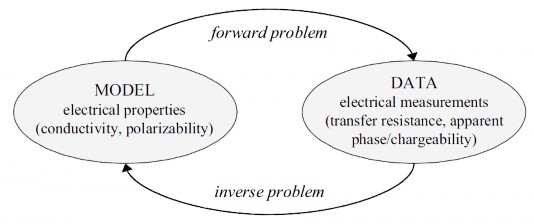
Figure 16 Electrical forward and inverse problems.

While the forward problem has a unique solution with each model and sources, it is different for the inverse problem.

When solving an inverse problem, three important questions must be answered:

1. Does the solution exist?

2. Is it unique?

3. Is it stable?

The question of the solution's existence is related to the mathematical formulation of the inverse problem. From the mathematical point of view, there could possibly be no adequate numerical model from the given model set which would fit our observed data. From the geophysical point of view, however, there should be some certain solution, since we study real geological structures of the earth's interior.

The question of the uniqueness of the solution can be illustrated by the

following formulae. Assume that we have two different models, m1 and m2 , and two

different sources,

s1 and s2 , which generate the same data d0

with the forward

modeling operator A :

A m1, s1 A m2 , s2

d0 ,

d0 .

In this case, it is impossible to distinguish these two models from the given

data. That is why the question of uniqueness is so important in inversion.

The question of solution stability is also a crucial one. Real geophysical data are always contaminated by some noises d . The question is whether the different between responses from different models is larger than the noise level. If the answer is not, it is impossible to distinguish these models from each other based on our data.

According to the French mathematician Hadamard [20], if all questions raised above have positive answer, the problem is said to be wellposed. Problems which are not wellposed are called illposed by Hadamard. Illposed problems may not have a solution or the solution is not unique or if a small change in the observed data would cause a large perturbation in the solution of the problem.

Hadamard considered illposed problems not mathematically or physically meaningful. However, most scientific problems, including geophysical ones are ill posed and it was subsequently found out that these problems are still meaningful and can be solved [26].

Foundations of the theory of illposed problems were developed by the Russian mathematician Andrei Tikhonov [13] in the middle of the 20th century. Tikhonov who is best known for his work on regularization of inverse problems also worked on

geophysical problems. He explains in detail how to solve the resistivity tomography problem in a simple case of 2layered medium. During the 1940s he collaborated with geophysicists and without the aid of computers they discovered large deposits of copper. As a result they were awarded a State Prize of Soviet Union.

An indepth book on the inverse problem topic in geophysics is [26].

With all common methods for solving the inverse problem, the forward problem has to be solved many times. It is therefore necessary to develop the forward module which can produce results with reasonable precision in acceptable time.

2.2 The geophysical model

The resistivity of a material is defined as the resistance in ohms between the opposite faces of a unit cube of the material. The SI (Système International) unit of resistivity is ohmmetre (ohm.m). If resistivity r is know, resistance can be computed by taking the integral of the formula:

R L,

with R being resistance, L being the length of the material and s being the cross sectional area.

In exploration geophysics, resistivity is a very important physical parameter that provides information about the mineral content and physical structure of rocks, and also about fluids in the rocks. Different materials have different resistivity value. The composition of the underground can therefore be studied by measuring the underground resistivities.

Electrical conductivity is the reciprocal (inverse) of electrical resistivity, and has the SI units of Siemens per meter (S.m1).

For the simplest case with a homogenous subsurface and a single point current source on the ground surface, the electrical potential varies inversely with the distance from the source (Figure 17):

V I .

2 R

The equipotential surfaces for this case are spherical surfaces radiating from the current electrode position.

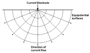
Figure 17 Homogenous subsurface with single point current source.

With two point sources one positive and one negative, we get

V I1

2 r1

where r1

electrodes.

and are distances of the point from the first and second current

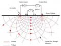
In most surveys, the potential difference between two points is measured. Two emitting electrodes, one positive, one negative, are used to inject the current into the ground. Two electrodes are receiving electrodes. The potential difference between them can be measured using a volt meter. The most used material for electrodes is stainless steel but others, such as copper and brass, are also used. A typical arrangement with four electrodes is shown in Figure 18.

The potential difference in the case of four electrodes over a homogenous half space is

V I

rAM

rBM

rAN

rBN

. (2.1)

Figure 18 shows a four electrode arrangement with the current source, four electrodes A, B, M, N (A is the positive source, B is the negative source, M and N are receiving electrodes), current meter, volt meter together with current flows and

Xem tất cả 65 trang.

Ngày đăng: 09/05/2022