A parallel implementation on modern hardware for geo electrical tomographical software

equipotential surfaces. If the half space is not homogenous, the value of computed from the above equation is the apparent resistivity.

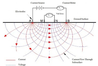
Figure 18 A four electrode arrangement.

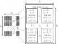
There are many types of electrode array. [6] provides details about each type of common electrode arrays. A few electrode configurations are shown on Figure 19.

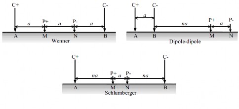
Figure 19 Example surface electrode configurations [11].

Different arrays have different depth of investigation, sensitivity to vertical and horizontal changes in the subsurface resistivity, horizontal data coverage and signal strength. It is therefore up to the geophysicists to choose the appropriate electrode array depending on survey objectives, spatial variability of electrical properties, access to suitable electrode site and equipment availability.

Có thể bạn quan tâm!

Xem toàn bộ 65 trang tài liệu này.

Figure 20 shows the difference in received signal between some electrode array types. Contours show relative contributions to the signal from unit volumes of homogeneous ground. Dashed lines indicate negative values.

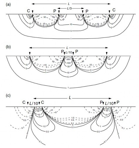
Figure 20 Signal contribution sections for a) Wenner array b) Schlumberger array c) dipoledipole arrays [7].

A reasonable first reaction to the measuring of resistivities shown in this figure is that useful resistivity surveys are impossible, as the contributions from regions close to the electrodes are very large. However, the variations in sign imply that a conductive nearsurface layer will in some places increase and in other places decrease the apparent resistivity. In homogeneous ground these effects can cancel quite precisely.

When a Wenner or dipole–dipole array is expanded, all the electrodes are moved and the contributions from nearsurface bodies vary from reading to reading.

With a Schlumberger array, nearsurface effects vary much less, provided that only the outer electrodes are moved, and for this reason the array is often preferred for depth sounding. However, offset techniques allow excellent results to be obtained with the Wenner.

The electrode array is moved together along the profile and the apparent resistivity is measured. Data points are collected for each electrode position. Data points at deeper layer are measured by repeating for array with larger width parameters.

In the past, geophysicists had to measure each data point manually but by the mid to late 1990s, most instrument manufacturers were able to offer multiplexed instruments, and in some cases multimeasurement channel hardware, thus enabling reduced survey time. Autonomous data acquisition systems are emerging and offer great potential for remote monitoring. From the collected data, a pseudosection of the underground apparent resistivity can be constructed. With each measurement, the potential difference is measured and the apparent resistivity is calculated using equation (2.1). This apparent resistivity provides a datum point. After all measurements are completed, we can produce an apparent resistivity model of the underground (Figure 21).

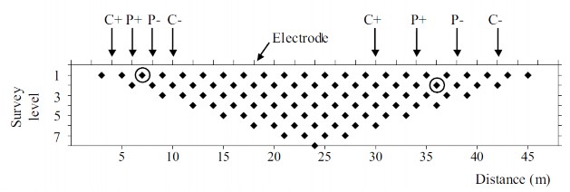
Figure 21 An example pseudosection [11].

2.3 The forward problem by differential method

Fully analytical methods have been used for simple cases of the forward modeling problem, such as a sphere in a homogenous medium or a vertical fault

between two areas each with a constant resistivity. However, this can not be applied to general cases. Here we present the forward problem using differential equations.

The input of the forward algorithm is a discretized mesh model of the subsurface in which each mesh cell is assigned a resistivity value. The most common model is a rectangular mesh while triangular meshes have also been proposed.

For the general 3D case the partial differential equation to be solved is

div

x, y, z grad V (x, y, z

I x xA

y yA

z zA

, (2.2)

where A is the point of current injection.

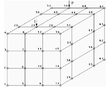
Figure 22 An example 3D mesh [5].

The boundary conditions are

V (x, y, z) must be continuous across each element boundary of the contrasting physical property distribution of σ (x, y).

the potential is zero at infinity

V 0 ,

there is no current leak into the air which means at the horizontal

boundary

V0 .

The equation can be solved using finite difference or finite element method with the above boundary conditions. The boundary condition at infinity is satisfied by expanding the mesh to a distance far enough. The result is a linear system of the form

Av = b ,

which can be solved using sparse linear solvers asA is a sparse matrix. Details on getting this linear system can be found in [9].

For the 2D case, the resistivity distribution is assumed to be constant in the y

direction.

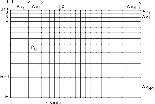
Figure 23 A 2D Mesh [5]

Applying the Fourier transform

V (x, k, z)

to equation (2.2) yields

V (x, y, z) cos(ky)dy ,

V V2 ~ I

x x y

z k V

2 x xA

z zA

(2.3)

with k being the wave number. This equation can be solved using the same method as (2.2). Once the result is obtained, the approximated inverse Fourier transform

V x, z

2n ~

i 0

x, k, z gi ,

is applied to get back V ( n is the number of wave numbers, weights for each wave number).

gi are the summation

An interesting problem is that although the wave number has to be theoretically continuous, in reality, we can only solve (2.3) for a limited number of wave numbers. The number of wave numbers should be minimized to speed up the computation but the accuracy must not be affected. A method for getting the optimal wave numbers and their Fourier inverses is detailed in [10]. The idea is to get the wave numbers from cases where the analytical solution to the forward problem equation is known.

Chapter 3 Software Implementation‌

3.1 Algorithms for solving large linear systems

For solving large linear systems, both iterative methods and direct methods can be used. While direct methods such as Gaussian elimination or LU decomposition give us an exact solution after a finite number of operations, iterative methods start with an initial solution and improve upon it after each iteration, obtaining a reasonably good approximation of the solution after a number of iterations.

For dense matrices, both direct and iterative methods are commonly used. With large sparse matrices, however, direct methods can become more costly in both memory footprint and implementation complexity as new nonzero elements can appear when using direct methods causing problems for storage and computation. As a result, iterative solvers are more common place for sparse linear systems. Iterative methods are also easier for finegrained parallelization.

In our case, we use the conjugate gradient method, a common iterative method for solving our linear systems. The Wikipedia article [14] provides a good amount of details on this method. Here we only present an overview of the conjugate gradient method.

Although all iterative methods obtain the results through a number of iterations, there are many differences in how the iterations are carried out. For the family of relaxation methods, the result of an iteration only depends on the result of the previous one. The conjugate gradient method and some other methods can use the result of all previous iterations for producing the result of an iteration for faster convergence.

Proper treatment of the theory behind iterative methods is a complicated subject. Below is the conjugate gradient method for solving the system

as presented in [14]:

Choose initial guess u0

Au f

(possibly the zero vector)

r0 f

p0 r0

Au0

for k

1,2,...

wk 1

Apk 1

αk 1

T 1rk 1

k 1 k 1

uk uk 1 αk 1pk 1

rk rk 1 αk 1wk 1

if rk is less than some tolerance then stop

βk 1

rTr

rT r

end for.

k k

zk βk

k 1 k 1

1pk 1

To increase convergence, a preconditioner M is often used. This is called the preconditioned conjugate gradient method. The preconditioner is a matrix that can provide an approximation of the matrix A . There are many types of preconditioners, including diagonal, incomplete Cholesky and incomplete LU. The above algorithm then becomes:

Choose initial guess u0

r0 f Au0

Solve Mz0 r0 p0 z0

for z0

for k

1,2,...

wk 1

Apk 1

αk 1

T 1rk 1

k 1 k 1

uk uk 1 αk 1pk 1

rk rk 1 αk 1wk 1

if rk is less than some tolerance then stop

Solve Mzk rk for zk

Xem tất cả 65 trang.

Ngày đăng: 09/05/2022