A parallel implementation on modern hardware for geo electrical tomographical software

βk 1

zTr

rT r

end for.

k k

zk βk

k 1 k 1

1pk 1

3.2 CPU implementation

For each wave number, a large number of linear systems have to be solved. In theory, this equals the number of data points which means that for each electrode arrangement, a linear system must be solved. This is the common method in most research articles [9], [10]. However, according the superposition property of the electrical field, the electrical potential caused by two electrodes is the sum of the two potential caused by each electrode:

v = v1 - v2 ,

where

v1 is the potential caused by the positive electrode and

v2 is the potential

caused by the negative electrode. As a result, the potential has to be calculated only for each electrode position and the results for each data point can be produced from the calculated results for single electrodes using equation (2.1). This means the number of linear systems we have to solve now only equals the number of electrodes, not the number of data points. For example, a survey with 100 electrodes can have more than 900 data points for a pseudosection depth of 10. With this notice, we can reduce the number of needed computations by a large magnitude.

Although the number of linear systems is large, they can be solved independently. Parallelization can therefore be done on a coarsegrain scale. In our software, Intel Threading Building Blocks [4] is used for parallelizing the code as this library is portable across platforms, provides good load balancing and has good documentation with a large user community. The loop over all the linear systems is parallelized using TBB’s parallel_for. We use the Matrix Template Library 4 by Open Systems Lab at Indiana University for solving each linear system. Running time for typical test cases are quite optimistic as near linear scale can be achieved. On our Core 2 Quad 9400 test system, for example, a speedup of 3.9x is observed.

3.2 Example Results

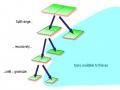
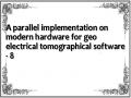
Surface

Block

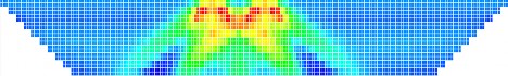
Here we present some results for common underground model using the Wenner alpha electrodes array. Each example contains two picture. The picture on top is the model. The picture below is the result after running the forward modeling module.

Environment

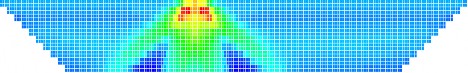
Figure 24 Example 1

Surface

Environment

Area with higher resistivity

Có thể bạn quan tâm!

Xem toàn bộ 65 trang tài liệu này.

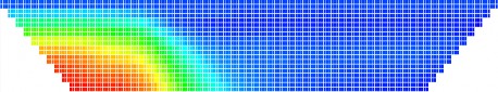
Figure 25 Example 2

Surface

Block 1

Block 2

Environment

Sur

Figure 26 Example 3

face

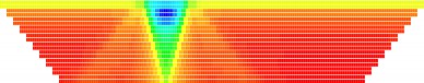
Figure 27 Example 4

3.3 GPU Implementation using CUDA

For the 2D case, the number of electrodes is often less than 1000. The above multicore CPU implementation can therefore be adequate for 2D surveys. However, for 3D surveys, the number of electrodes can be a few thousands or more and the 3D mesh is significantly larger than the 2D mesh. It is therefore essential to get more performance increase for large data sets. Traditionally, this has been done using clusters, which are expensive and inconvenient for ordinary users. At the moment, we are experimenting with porting computationally expensive parts of the program to run on the GPU.

It can be seen form chapter 1 that GPU has a very different model of execution from CPU. The memory hierarchy is also different. This lead to more work in porting a program from CPU to GPU.

Choosing the right matrix format is an important first step. There are a few common sparse matrix formats to choose from.

For dense matrices, most elements are nonzero and the storage format often stores all the matrix elements in columnmajor or rowmajor form. For sparse matrices, because of the fact that a large number of elements are zero, it is more efficient to store only the nonzero ones to save space and increase computation speed. This requires for more complicated storage scheme than dense matrices.

Some common sparse matrix formats are

Compressed Sparse Row (CSR) format: a vector contains the entire matrix elements in which the elements in the same row are next to each other, rows are placed according to their position in the matrix. A second vector contains the columns of the elements. The third vector contains the start of each row in the first vector.

1	7	0	0
0	2	8	0
5	0	3	9
0	6	0	4
0	2	4	7 9

For example the matrix

has the CSR presentation

indices

ptr

0 1 1 2 0

2 3 1 3

data

1 7 2 8

5 3 9 6 4 .

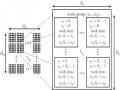
Diagonal format: every diagonal of the matrix that has a non zero is stored. Zeros are padded in so every diagonal has the same length. This is most suitable for matrices produced by finite differencing.

1	7	0	0
0	2	8	0
5	0	3	9
0	6	0	4

For example, the matrix

has the diagonal presentation

*	1	7
*	2	8
5	3	9
6	4	*
	2 0		1 .

data

offsets

ELL format: every row is assumed to have no more than a fixed number of nonzeros. Zeros are padded in if the row has fewer nonzeros. The column of each element is also explicitly stored.

For example, the matrix

Α0

has the ELL presentation:

1 7 *

7 0 0

2 8 0

0 3 9

6 0 4

0 1 *

data

2 8 *

indices

1 2 * .

5	3	9	0	2	3
6	4	*	1	3	*

1	7	0	0
0	2	8	0
5	0	3	9
0	6	0	4

COO format: both the coordinate and the value of the element are stored. For example, the matrix

has COO presentation

row

0	0	1	1	2	2	2	3	3
col	0	1	1	2	0	2	3	1	3
data	1	7	2	8	5	3	9	6	4 .

Many other formats have also been proposed. Some are hybrid of the existing types, some are completely new format.

There are many other types of matrix data formats. Finding the appropriate format for specific parallel architectures requires a much deeper understanding of the inner of hardware and parallel algorithms. This should be an interesting subject for further research.

In the CPU implementation, we use the CSR format as it is the most common in matrix libraries and supported by many solvers. However, this format is inefficient for GPU as memory access in the matrixvector multiplication kernel is not contiguous, which significantly slow down GPU computation. As we use finite difference in our mesh, we use the diagonal format to enable contiguous memory access.

We have also applied some common optimizations for GPU kernels. Attention has been paid to the use of shared memory within GPU threads in the same block to avoid access to the slower global memory. This alone proves to be quite effective in optimizing for GPU. We also tried to keep the processing on the GPU for as long as possible to avoid long memory transfer time between GPU and CPU. For small cases, grouping smaller matrices into larger ones can help get more bandwidth as the bandwidth is often underutilized for these cases.

Porting the whole computation part of the program to GPU is an ongoing task that requires more time to complete. Below are preliminary results for comparison between CPU and GPU conjugate gradient method with diagonal preconditioner after some optimization on the GPU kernels.

The CPU code is run on a Core 2 Quad Q9400 CPU (2.66 GHz, 6 MB cache). The GPU code is run on an MSI Nvidia 9800GT GPU (600 MHz core clock, 1375 MHz shader clock, 512 MB GDDR3). The time is measured for 2D survery datasets. However, with 3200 electrodes, the amount of computation is quite the same as large 3D datasets. Memory copy operation between CPU and GPU is already included in the GPU execution timing to provide real comparison between GPU time and CPU time.

2000

1500

1000

CPU sequential CPU parallel

GPU

500

100

200 400 800 1600 3200

Numbe r of e lectrode s

Running time (s)

Figure 28 Running time for different implementations (CPU sequential time is not measured after 800 electrodes because of long running time).

It can be seen that for large datasets, the GPU shows up to more than 6x speed up over a 4core CPU. This is quite promising for an old GPU such as the Geforce 9800. The GPU also has a 75W TDP compared to the 120W TDP of the CPU. The speed up can be improved in the future as there is still much room for improvement in our GPU kernel. GPUs are also getting much faster with each generation with better compilers and tools. GPU computing can therefore be a viable option for processing large 3D survey datasets with a great amount of speed up over CPU computing.

We are currently working on a multiGPU implementation. This requires more research into the problem of load balancing between different GPUs. Using a cluster with multiGPU nodes is also an interesting research area which has the potential to solve larger problems at lower cost and power consumption.

CONCLUSION‌

In the first phase of our project, we have developed the forward module for the resistivity tomography problem. Our implementation can run on multicore CPUs and GPUs. Future versions may see new modules for resistivity inversion and other geophysical features. We are also working on making our code more efficient and more scalable over different kinds of architecture.

Xem tất cả 65 trang.

Ngày đăng: 09/05/2022