A parallel implementation on modern hardware for geo electrical tomographical software - 2

Instruction­Level Parallel (Fined­Grained Control Parallelism) Process­Level Parallel (Coarse­Grained Control Parallelism) Data Parallel (Data Parallelism)

These categories are not exclusive of each other. A hardware device (such as

the CPU) can belong to all these three groups.

1.1.1 Instruction­Level Parallel Architectures

There are two common kinds of instruction­level parallel architecture.

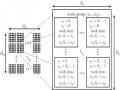
The first is superscalar pipelined architectures which subdivide the execution of each machine instruction into a number of stages. As short stages allow for high clock frequencies, the recent trend is to use longer pipeline. For example the Pentium 4 uses a 20­stage pipeline and the latest Pentium 4 core contains a 31­stage pipeline.

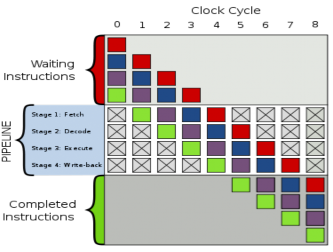
Figure 1 Generic 4­stage pipeline; the colored boxes represent instructions independent of each other [21].

A common problem with these pipelines is branching. When branches happen, the processor has to wait until the branch finishes fetching the next instruction. A branch prediction unit is put into the CPU to guess which branch would be executed. However, if branches are predicted poorly, the performance penalty can be high. Some programming techniques to make branches in code more predictable for hardware can be found in [2]. Programming tools such as Intel VTune Performance Analyzer can be of great help in profiling programs for missed branch predictions.

Có thể bạn quan tâm!

• A parallel implementation on modern hardware for geo electrical tomographical software - 1
• Programming Tools For Scientific Computing On Personal Desktop Systems
• A parallel implementation on modern hardware for geo electrical tomographical software - 4
• A parallel implementation on modern hardware for geo electrical tomographical software - 5

Xem toàn bộ 65 trang tài liệu này.

The second kind of instruction­level parallel architecture is VLIW (very long instruction word) architectures. A very long instruction word usually controls 5 to 30 replicated execution units. An example of VLIW architecture is the Intel Itanium processor [23]. As of 2009, Itanium processors can execute up to six instructions per cycle. For ordinary architectures, superscalar execution and out­of­order execution is used to speed up computing. This increases hardware complexity. The processor must decide at runtime whether instruction parts are independent so that they can be executed simultaneously. In VLIW architectures, this is decided at compile time. This shifts the hardware complexity to software complexity. All operations in one instruction must be independent so efficient code generation is a hard task for compilers. The problem of writing compilers and porting legacy software to the new architectures make the Itanium architecture unpopular.

1.1.2 Process­Level Parallel Architectures

Process­level parallel architectures are architectures that exploit coarse­grained control parallelism in loops, functions or complete programs. They replicate complete asynchronously executing processors to increase execution bandwidth and, hence, fit the multiple­instruction­multiple­data (MIMD) paradigm.

Until a few years ago, these architectures comprised of multiprocessors and multicomputers.

A multiprocessor uses a shared memory address space for all processors. There are two kinds of multiprocessors:

Symmetric Multiprocessor or SMP computers: the cost of accessing an address in memory is the same for each processor. Furthermore, the processors are all equal in the eyes of the operation system.

Non­uniform Memory Architecture or NUMA computers: the cost of accessing a given address in memory varies from one processor to another.

In a multicomputer, each processor has its own local memory. Access to remote memory requires explicit message passing over the interconnection network. They are also called distributed memory architectures or message­passing architectures. An example is cluster system. A cluster consists of many computing nodes, which can be built using high­performance hardware or commodity desktop hardware. All the nodes

in a cluster are connected via Infiniband or Gigabit Ethernet. Big clusters can have thousands of nodes with special topologies for interconnect. Cluster is currently the only affordable way for large scale supercomputing at the level of hundreds of teraflops or more.

Figure 2 Example SMP system (left) and NUMA system (right)

A recent derivative of cluster computing is grid computing [19]. While traditional clusters often consist of similar nodes close to each other, grids will incorporate heterogeneous collections of computers, possibly distributed geographically. They are, therefore, optimized for workloads containing many independent packets of work. The two biggest grid computing network is Folding@home and SETI@home (BOINC). Both have the computing capability of a few petaflops while the most powerful traditional cluster can barely reach over 1 petaflops.

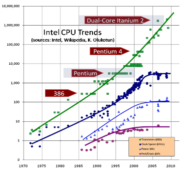
Figure 3 Intel CPU trends [12].

The most notable change to process­level parallel architectures happened in the last few years. Figure 3 shows that although the number of transistors a CPU contains still increases according to Moore’s law (which means doubling every 18 months), the clock speed has virtually stopped rising due to heating and manufacturing problems. CPU manufacturers have now turned to adding more cores to a single CPU while the clock speed stays the same or decreases. An individual core is a distinct processing element and is basically the same as a CPU in an older single­core PC. A multi­core chip can now be considered a SMP MIMD parallel processor. A multi­core chip can run at lower clock speed and therefore consumes less power but still has increases in processing power.

The latest Intel Core i7­980 (Gulftown) CPU has 6 cores and 12 MB of cache. With hyper­threading it can support up to 12 hardware threads. Future multi­core CPU generations may have 8, 16 or even 32 cores in the next few years. These new architectures, especially in multi­processor node, can provide the level of parallelism that has been only available to cluster systems.

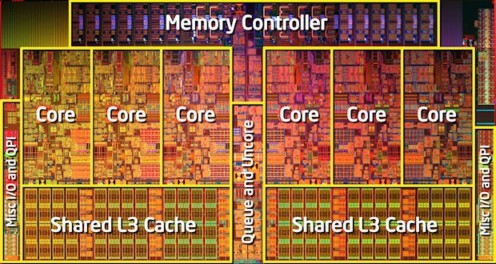
Figure 4 Intel Gulftown CPU .

1.1.3 Data parallel architectures

Data parallel architectures appeared very soon on the history of computing. They utilize data parallelism to increase execution bandwidth. Data parallelism is common in many scientific and engineering tasks where a single operation is applied to a whole data set, usually a vector or a matrix. This allows applications to exhibit a large amount of independent parallel workloads. Both pipelining and replication have been applied to hardware to utilize data parallelism.

Pipelined vector processors such as the Cray 1 [15], operates on vectors rather than scalar. After the instruction is decoded, vectors of data stream directly from memory into the pipelined functional units. Separate pipelines can be chained together to get higher performance. The translation of sequential code into vector instructions is called vectorization. A vectorizing compiler played a crucial role in programming for vector processors. This has significantly pushed the maturity of compilers in generating efficient parallel code.

Through replication, processor arrays can utilize data parallelism as a single control unit can order a large number of simple processing elements to operate the same instruction on different data elements. These massively parallel supercomputers fit into the single­instruction­multiple­data (SIMD) paradigm.

Although both of the kinds of supercomputers mentioned above have virtually disappeared from common use, they are precursors for current data parallel architectures, most notably the CPU SIMD processing and GPUs.

The CPU SIMD extension instruction set for Intel CPUs include MMX, SSE, SSE2, SSE3, SSE4 and AVX. They allow the CPU to use a single operation to operate on several data elements simultaneously. AVX, the latest extension instruction set is expected to be implemented on both Intel and AMD products in 2010 and 2011. With AVX, the size of SIMD vector register is increased from 128­bit to 256­bit, which means the CPU can operate on 8 single­precision or 4 double­precision floating point numbers during one instruction. CPU SIMD processing has been used widely by programmers in many applications such as multimedia and encryption and compiler code generation for these architectures are now considerably good. Even when multicore CPUs are popular, understanding SIMD extensions is still vital for optimizing program execution on each CPU core. A good handbook on utilizing software vectorization is [1].

However, graphics processing units (GPUs) are perhaps the hardware with the most dramatic growth in processing power over the last few years.

Graphics chips started as fixed function graphics pipelines. Over the years, these graphics chips became increasingly programmable with newer graphics API and shaders. In the 1999­2000 timeframe, computer scientists in particular, along with researchers in fields such as medical imaging and electromagnetic started using GPUs for running general purpose computational applications. They found the excellent floating point performance in GPUs led to a huge performance boost for a range of scientific applications. This was the advent of the movement called GPGPU or General Purpose computing on GPUs.

With the advent of programming languages such as CUDA and OpenCL, GPUs are now easier to program. With the processing power of a few Teraflops, GPUs are now massively parallel processors at a much smaller scale. They are now also termed stream processors as data is streamed directly from memory into the execution units without the latency like the CPUs. As can be seen in Figure 5, GPUs have currently outpaced CPUs many times in both speed and bandwidth.

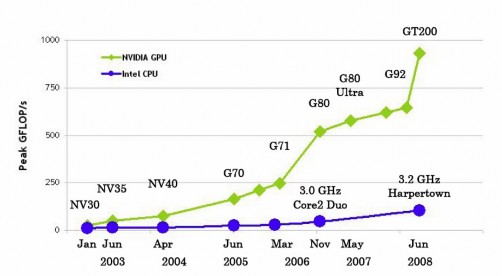
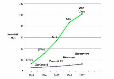
Figure 5 Comparison between CPU and GPU speed and bandwidth (CUDA programming Guide) [8].

The two most notable GPU architectures now are the ATI Radeon 5870 (Cypress) and Nvidia GF100 (Fermi) processor.

The Radeon 5870 processor has 20 SIMD engines, each of which has 16 thread processors inside of it. Each of those thread processors has five arithmetic logic units, or ALUs. With a total of 1600 stream processors and a clock speed of 850 MHz, Radeon 5870 has the single­precision computing power of 2.72 Tflops while top of the line CPU still has processing power counted in Gflops. Double­precision computing is done at one fifth of the rate for single­precision, at 544 Gflops. This card supports both

OpenCL and DirectCompute. The double version, the Radeon 5970 (Hemlock) dual graphics processor has a single­precision computing power of 4.7 Tflops in a graphics card at a thermal envelope of less than 300 W. Custom over clocked versions made by graphics card manufacturer can even offer much more computing power than the original version.

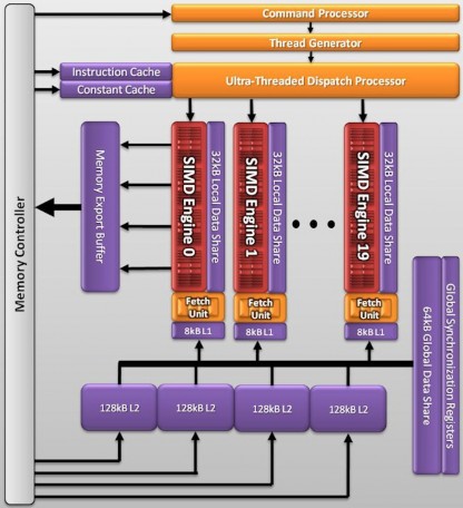
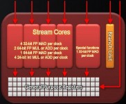
Figure 6 ATI Radeon 5870 (Cypress) graphics processor

The Nvidia GF100 processor has 3 billion transistors with 15 SM (Shader Multiprocessor) units, each has 32 shader cores or CUDA processor compared to 8 of previous Nvidia GPUs. Each CUDA processor has a fully pipelined integer arithmetic logic unit and floating point unit with better standard conformance and fused multiply­ add instruction for both single and double precision. The integer precision was raised from 24 bit to 32 bit so multi­instruction emulation is no longer required. Special function units in each SM can execute transcendental instructions such as sin, cosine, reciprocal and square root.