Khả năng sinh trưởng, sản xuất thịt của bò lai sind, F1 brahman × lai sind và F1 charolais × lai sind nuôi tại Đăk Lăk

BÊ LAI F1(BRAHMAN × LAI SIND), 2 THÁNG TUỔI ĐẠT 70 KG

BÊ LAI F1(BRAHMAN × LAI SIND), 12 THÁNG TUỔI

BÊ LAI F1(CHAROLAIS × LAI SIND) TẠI EAKAR, ĐĂK LĂK

BÊ LAI F1(CHAROLAIS × LAI SIND) TẠI HỘI CHỢ BÒ HUYỆN EAKAR TỈNH ĐĂK LĂK

ẢNH MÀU SẮC THỊT CỦA BÒ LAI SIND BẢO QUẢN LÚC 8 NGÀY

ẢNH MÀU SẮC THỊT CỦA BÒ LAI F1 (BRAHMAN × LAI SIND) BẢO QUẢN LÚC 8 NGÀY

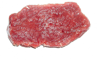
ẢNH MÀU SẮC THỊT CỦA BÒ LAI F1 (CHAROLAIS × LAI SIND) BẢO QUẢN LÚC 8 NGÀY

KẾT QUẢ CHẠY HÀM GOMPERTZ BẰNG PHƯƠNG PHÁP MARQUART TRÊN PHẦN MỀM STARTGRAPHIS CENTURION IV

Nonlinear Regression - Lai Sind NNH

Dependent variable: Kg Independent variables:

Tháng

Function to be estimated: m*exp(-a*exp(-b*Tháng)) Initial parameter estimates:

m = 100.0

a = 1.0

b = 0.1

Estimation method: Marquardt

Estimation stopped due to convergence of residual sum of squares. Number of iterations: 5

Number of function calls: 22

Estimation Results

		Asymptotic	95.0%
		Asymptotic	Confidence	Interval
Parameter	Estimate	Standard Error	Lower	Upper
m	267.261	2.57414	262.216	272.306
a	2.41752	0.0257114	2.36713	2.46792
b	0.112467	0.00213622	0.10828	0.116654

Có thể bạn quan tâm!

Xem toàn bộ 170 trang tài liệu này.

Analysis of Variance

Source

Sum of Squares	Df	Mean Square
Model	2.44495E7	3	8.14982E6
Residual	171782.	1137	151.083
Total	2.46212E7	1140
Total (Corr.)	5.57748E6	1139

R-Squared = 96.9201 percent

R-Squared (adjusted for d.f.) = 96.9147 percent Standard Error of Est. = 12.2916

Mean absolute error = 9.902 Durbin-Watson statistic = 0.608713

Lag 1 residual autocorrelation = 0.694243

Residual Analysis

Estimation	Validation
n	1140
MSE	151.083
MAE	9.902
MAPE	10.9383
ME	-0.252355
MPE	-4.26433

The StatAdvisor

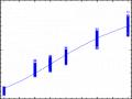
The output shows the results of fitting a nonlinear regression model to describe the relationship between Kg and 1 independent variables. The equation of the fitted model is

Kg = 267.261*exp(-2.41752*exp(-0.112467*Tháng))

In performing the fit, the estimation process terminated successully after 5 iterations, at which point the estimated coefficients appeared to converge to the current estimates.

The R-Squared statistic indicates that the model as fitted explains 96.9201% of the variability in Kg. The adjusted R- Squared statistic, which is more suitable for comparing models with different numbers of independent variables, is

96.9147%. The standard error of the estimate shows the standard deviation of the residuals to be 12.2916. This value can be used to construct prediction limits for new observations by selecting the Forecasts option from the text menu. The mean absolute error (MAE) of 9.902 is the average value of the residuals. The Durbin-Watson (DW) statistic tests the residuals to determine if there is any significant correlation based on the order in which they occur in your data file.

The output also shows aymptotic 95.0% confidence intervals for each of the unknown parameters. These intervals are approximate and most accurate for large sample sizes. You can determine whether or not an estimate is statistically significant by examining each interval to see whether it contains the value 0. Intervals covering 0 correspond to coefficients which may well be removed form the model without hurting the fit substantially.

Plot of Fitted Model

300

250

200

150

100

0 3 6 9 12 15 18 21 24

Tháng

Nonlinear Regression - F1(Bra × LS) NNH

Dependent variable: Kg Independent variables:

Thang

Function to be estimated: m*exp(-a*exp(-b*Thang)) Initial parameter estimates:

m = 100.0

a = 1.0

b = 0.1

Estimation method: Marquardt

Estimation stopped due to convergence of residual sum of squares. Number of iterations: 6

Number of function calls: 27

Estimation Results

		Asymptotic	95.0%
		Asymptotic	Confidence	Interval
Parameter	Estimate	Standard Error	Lower	Upper
m	333.643	4.09445	325.618	341.668
a	2.35868	0.0233789	2.31286	2.40451
b	0.101279	0.00218984	0.0969873	0.105571

Analysis of Variance

Source

Sum of Squares	Df	Mean Square
Model	3.22511E7	3	1.07504E7
Residual	245846.	1077	228.269
Total	3.24969E7	1080
Total (Corr.)	7.37714E6	1079

R-Squared = 96.6675 percent

R-Squared (adjusted for d.f.) = 96.6613 percent Standard Error of Est. = 15.1086

Mean absolute error = 12.5891 Durbin-Watson statistic = 0.456049

Lag 1 residual autocorrelation = 0.771676

Residual Analysis

Estimation	Validation
n	1080
MSE	228.269
MAE	12.5891
MAPE	14.2699
ME	-0.487939
MPE	-6.82747

The StatAdvisor

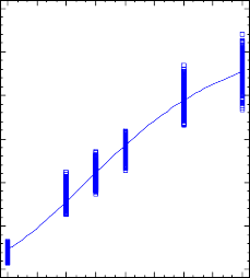
The output shows the results of fitting a nonlinear regression model to describe the relationship between Kg and 1 independent variables. The equation of the fitted model is

Kg = 333.643*exp(-2.35868*exp(-0.101279*Thang))

In performing the fit, the estimation process terminated successully after 6 iterations, at which point the estimated coefficients appeared to converge to the current estimates.

The R-Squared statistic indicates that the model as fitted explains 96.6675% of the variability in Kg. The adjusted R- Squared statistic, which is more suitable for comparing models with different numbers of independent variables, is 96.6613%. The standard error of the estimate shows the standard deviation of the residuals to be 15.1086. This value can be used to construct prediction limits for new observations by selecting the Forecasts option from the text menu. The mean absolute error (MAE) of 12.5891 is the average value of the residuals. The Durbin-Watson (DW) statistic tests the

residuals to determine if there is any significant correlation based on the order in which they occur in your data file.

Plot of Fitted Model

400

300

200

100

0 3 6 9 12 15 18 21 24

Thang

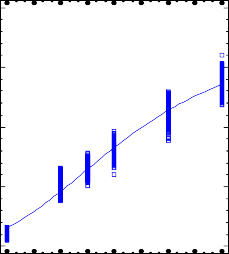
Nonlinear Regression - F1 (Char × LS) NNH

Dependent variable: Kg Independent variables:

Thang

Function to be estimated: m*exp(-a*exp(-b*Thang)) Initial parameter estimates:

m = 100.0

a = 1.0

b = 0.1

Estimation method: Marquardt

Estimation stopped due to convergence of residual sum of squares. Number of iterations: 6

Number of function calls: 28

Estimation Results

		Asymptotic	95.0%
		Asymptotic	Confidence	Interval
Parameter	Estimate	Standard Error	Lower	Upper
m	383.999	4.98571	374.227	393.771
a	2.43216	0.0210278	2.39095	2.47337
b	0.0953172	0.00199682	0.0914035	0.0992309

Analysis of Variance

Source

Sum of Squares	Df	Mean Square
Model	4.03042E7	3	1.34347E7
Residual	282320.	1137	248.302
Total	4.05865E7	1140
Total (Corr.)	9.57182E6	1139

R-Squared = 97.0505 percent

R-Squared (adjusted for d.f.) = 97.0453 percent Standard Error of Est. = 15.7576

Mean absolute error = 13.1394 Durbin-Watson statistic = 0.377343

Lag 1 residual autocorrelation = 0.810484

Residual Analysis

Estimation	Validation
n	1140
MSE	248.302
MAE	13.1394
MAPE	14.779
ME	-0.52582
MPE	-7.35733

The StatAdvisor

The output shows the results of fitting a nonlinear regression model to describe the relationship between Kg and 1 independent variables. The equation of the fitted model is

Kg = 383.999*exp(-2.43216*exp(-0.0953172*Thang))

In performing the fit, the estimation process terminated successully after 6 iterations, at which point the estimated coefficients appeared to converge to the current estimates.

The R-Squared statistic indicates that the model as fitted explains 97.0505% of the variability in Kg. The adjusted R- Squared statistic, which is more suitable for comparing models with different numbers of independent variables, is 97.0453%. The standard error of the estimate shows the standard deviation of the residuals to be 15.7576. This value can be used to construct prediction limits for new observations by selecting the Forecasts option from the text menu. The mean absolute error (MAE) of 13.1394 is the average value of the residuals. The Durbin-Watson (DW) statistic tests the

Xem tất cả 170 trang.

Ngày đăng: 10/11/2022