residuals to determine if there is any significant correlation based on the order in which they occur in your data file.
The output also shows aymptotic 95.0% confidence intervals for each of the unknown parameters. These intervals are approximate and most accurate for large sample sizes. You can determine whether or not an estimate is statistically significant by examining each interval to see whether it contains the value 0. Intervals covering 0 correspond to coefficients which may well be removed form the model without hurting the fit substantially.
Plot of Fitted Model
400
300
Kg
200
100
0
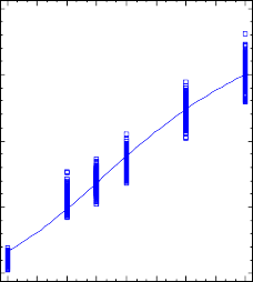
0 3 6 9 12 15 18 21 24
Thang
Nonlinear Regression - Lai Sind NTD
Dependent variable: Kg Independent variables:
Tháng
Function to be estimated: m*exp(-a*exp(-b*Tháng)) Initial parameter estimates:
m = 100.0
a = 1.0
b = 0.1
Estimation method: Marquardt
Estimation stopped due to convergence of residual sum of squares. Number of iterations: 7
Number of function calls: 33
Estimation Results
Asymptotic | 95.0% | |||
Asymptotic | Confidence | Interval | ||
Parameter | Estimate | Standard Error | Lower | Upper |
m | 350.379 | 9.47535 | 331.711 | 369.046 |
a | 2.60163 | 0.0418526 | 2.51917 | 2.68408 |
b | 0.0925204 | 0.00373819 | 0.0851559 | 0.0998849 |
Có thể bạn quan tâm!
-

 Phạm Thế Huệ (1997), Nghiên Cứu Một Số Tính Trạng Năng Suất Chủ Yếu Của Bò Địa Phương Và Bò Lai F1 (Red Sindhi × Bò Địa Phương) Tại Đăk Lăk, Luận
 -
 Khả năng sinh trưởng, sản xuất thịt của bò lai sind, F1 brahman × lai sind và F1 charolais × lai sind nuôi tại Đăk Lăk - 19
 -
 Khả năng sinh trưởng, sản xuất thịt của bò lai sind, F1 brahman × lai sind và F1 charolais × lai sind nuôi tại Đăk Lăk - 20
Xem toàn bộ 170 trang tài liệu này.
Analysis of Variance
Sum of Squares | Df | Mean Square | |
Model | 6.29082E6 | 3 | 2.09694E6 |
Residual | 32798.5 | 236 | 138.977 |
Total | 6.32362E6 | 239 | |
Total (Corr.) | 1.59501E6 | 238 |
R-Squared = 97.9437 percent
R-Squared (adjusted for d.f.) = 97.9263 percent Standard Error of Est. = 11.7888
Mean absolute error = 9.61235 Durbin-Watson statistic = 0.633805
Lag 1 residual autocorrelation = 0.674314
Residual Analysis
Estimation | Validation | |
n | 239 | |
MSE | 138.977 | |
MAE | 9.61235 | |
MAPE | 12.5865 | |
ME | -0.397958 | |
MPE | -6.15615 |
The StatAdvisor
The output shows the results of fitting a nonlinear regression model to describe the relationship between Kg and 1 independent variables. The equation of the fitted model is
Kg = 350.379*exp(-2.60163*exp(-0.0925204*Tháng))
In performing the fit, the estimation process terminated successully after 7 iterations, at which point the estimated coefficients appeared to converge to the current estimates.
The R-Squared statistic indicates that the model as fitted explains 97.9437% of the variability in Kg. The adjusted R- Squared statistic, which is more suitable for comparing models with different numbers of independent variables, is 97.9263%. The standard error of the estimate shows the standard deviation of the residuals to be 11.7888. This value can be used to construct prediction limits for new observations by selecting the Forecasts option from the text menu. The mean absolute error (MAE) of 9.61235 is the average value of the residuals. The Durbin-Watson (DW) statistic tests the
residuals to determine if there is any significant correlation based on the order in which they occur in your data file.
The output also shows aymptotic 95.0% confidence intervals for each of the unknown parameters. These intervals are approximate and most accurate for large sample sizes. You can determine whether or not an estimate is statistically significant by examining each interval to see whether it contains the value 0. Intervals covering 0 correspond to coefficients which may well be removed form the model without hurting the fit substantially.
Plot of Fitted Model
300
250
200
Kg
150
100
50
0
0 3 6 9 12 15 18 21 24
Tháng
Nonlinear Regression - F1(Bra × LS) NTD
Dependent variable: Kg Independent variables:
Tháng
Function to be estimated: m*exp(-a*exp(-b*Tháng)) Initial parameter estimates:
m = 100.0
a = 1.0
b = 0.1
Estimation method: Marquardt
Estimation stopped due to convergence of residual sum of squares. Number of iterations: 7
Number of function calls: 33
Estimation Results
Asymptotic | 95.0% | |||
Asymptotic | Confidence | Interval | ||
Parameter | Estimate | Standard Error | Lower | Upper |
m | 401.478 | 13.4843 | 374.914 | 428.043 |
a | 2.50368 | 0.0519627 | 2.40131 | 2.60605 |
b | 0.0934432 | 0.00485186 | 0.0838849 | 0.103001 |
Analysis of Variance
Sum of Squares | Df | Mean Square | |
Model | 8.74683E6 | 3 | 2.91561E6 |
Residual | 76604.9 | 237 | 323.227 |
Total | 8.82344E6 | 240 | |
Total (Corr.) | 2.16643E6 | 239 |
R-Squared = 96.464 percent
R-Squared (adjusted for d.f.) = 96.4342 percent Standard Error of Est. = 17.9785
Mean absolute error = 14.9868 Durbin-Watson statistic = 0.464853
Lag 1 residual autocorrelation = 0.764558
Residual Analysis
Estimation | Validation | |
n | 240 | |
MSE | 323.227 | |
MAE | 14.9868 | |
MAPE | 15.3557 | |
ME | -0.568747 | |
MPE | -7.56073 |
The StatAdvisor
The output shows the results of fitting a nonlinear regression model to describe the relationship between Kg and 1 independent variables. The equation of the fitted model is
Kg = 401.478*exp(-2.50368*exp(-0.0934432*Tháng))
In performing the fit, the estimation process terminated successully after 7 iterations, at which point the estimated coefficients appeared to converge to the current estimates.
The R-Squared statistic indicates that the model as fitted explains 96.464% of the variability in Kg. The adjusted R- Squared statistic, which is more suitable for comparing models with different numbers of independent variables, is 96.4342%. The standard error of the estimate shows the standard deviation of the residuals to be 17.9785. This value can be used to construct prediction limits for new observations by selecting the Forecasts option from the text menu. The mean absolute error (MAE) of 14.9868 is the average value of the residuals. The Durbin-Watson (DW) statistic tests the
residuals to determine if there is any significant correlation based on the order in which they occur in your data file.
The output also shows aymptotic 95.0% confidence intervals for each of the unknown parameters. These intervals are approximate and most accurate for large sample sizes. You can determine whether or not an estimate is statistically significant by examining each interval to see whether it contains the value 0. Intervals covering 0 correspond to coefficients which may well be removed form the model without hurting the fit substantially.
Plot of Fitted Model
400
300
Kg
200
100
0
0 3 6 9 12 15 18 21 24
Tháng
Nonlinear Regression - F1(Char × LS) NTD
Dependent variable: Kg Independent variables:
Tháng
Function to be estimated: m*exp(-a*exp(-b*Tháng)) Initial parameter estimates:
m = 100.0
a = 1.0
b = 0.1
Estimation method: Marquardt
Estimation stopped due to convergence of residual sum of squares. Number of iterations: 8
Number of function calls: 38
Estimation Results
Asymptotic | 95.0% | |||
Asymptotic | Confidence | Interval | ||
Parameter | Estimate | Standard Error | Lower | Upper |
m | 418.902 | 9.87592 | 399.446 | 438.358 |
a | 2.58998 | 0.0473538 | 2.4967 | 2.68327 |
b | 0.100544 | 0.00392725 | 0.0928075 | 0.108281 |
Analysis of Variance
Sum of Squares | Df | Mean Square | |
Model | 1.02258E7 | 3 | 3.4086E6 |
Residual | 55535.8 | 237 | 234.328 |
Total | 1.02813E7 | 240 | |
Total (Corr.) | 2.55602E6 | 239 |
R-Squared = 97.8273 percent
R-Squared (adjusted for d.f.) = 97.8089 percent Standard Error of Est. = 15.3078
Mean absolute error = 12.3686 Durbin-Watson statistic = 0.675345
Lag 1 residual autocorrelation = 0.661407
Residual Analysis
Estimation | Validation | |
n | 240 | |
MSE | 234.328 | |
MAE | 12.3686 | |
MAPE | 12.5273 | |
ME | -0.462302 | |
MPE | -5.9931 |
The StatAdvisor
The output shows the results of fitting a nonlinear regression model to describe the relationship between Kg and 1 independent variables. The equation of the fitted model is
Kg = 418.902*exp(-2.58998*exp(-0.100544*Tháng))
In performing the fit, the estimation process terminated successully after 8 iterations, at which point the estimated coefficients appeared to converge to the current estimates.
The R-Squared statistic indicates that the model as fitted explains 97.8273% of the variability in Kg. The adjusted R- Squared statistic, which is more suitable for comparing models with different numbers of independent variables, is 97.8089%. The standard error of the estimate shows the standard deviation of the residuals to be 15.3078. This value can be used to construct prediction limits for new observations by selecting the Forecasts option from the text menu. The mean absolute error (MAE) of 12.3686 is the average value of the residuals. The Durbin-Watson (DW) statistic tests the
residuals to determine if there is any significant correlation based on the order in which they occur in your data file.
The output also shows aymptotic 95.0% confidence intervals for each of the unknown parameters. These intervals are approximate and most accurate for large sample sizes. You can determine whether or not an estimate is statistically significant by examining each interval to see whether it contains the value 0. Intervals covering 0 correspond to coefficients which may well be removed form the model without hurting the fit substantially.
Plot of Fitted Model
400
300
Kg
200
100
0
0 3 6 9 12 15 18 21 24
Tháng