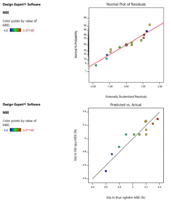
P8. KẾT QUẢ PHÂN TÍCH MEE THEO PHẦN MỀM DESIGN EXPERT
ANOVA for Quadratic model
Response 2: MEE
Source Sum of Squares df Mean Square F-value p-value
0.5834 | 5 | 0.1167 | 8.61 | 0.0067 | significant | |
A-C | 0.2376 | 1 | 0.2376 | 17.54 | 0.0041 | |
B-t | 0.1510 | 1 | 0.1510 | 11.15 | 0.0124 | |
AB | 0.1899 | 1 | 0.1899 | 14.02 | 0.0072 | |
A² | 0.0044 | 1 | 0.0044 | 0.3252 | 0.5863 | |
B² | 0.0001 | 1 | 0.0001 | 0.0100 | 0.9232 | |
Residual | 0.0948 | 7 | 0.0135 | |||
Lack of Fit | 0.0449 | 3 | 0.0150 | 1.20 | 0.4167 | not significant |
Pure Error | 0.0499 | 4 | 0.0125 | |||
Cor Total | 0.6782 | 12 |
Có thể bạn quan tâm!
-
 Nâng cao tính kỵ nước và chống tia uv cho gỗ Bồ đề Styrax tonkinensis bằng công nghệ phủ ZnO - 17
 -
 Nâng cao tính kỵ nước và chống tia uv cho gỗ Bồ đề Styrax tonkinensis bằng công nghệ phủ ZnO - 18
 -
 Nâng cao tính kỵ nước và chống tia uv cho gỗ Bồ đề Styrax tonkinensis bằng công nghệ phủ ZnO - 19
 -
 Nâng cao tính kỵ nước và chống tia uv cho gỗ Bồ đề Styrax tonkinensis bằng công nghệ phủ ZnO - 21
Xem toàn bộ 174 trang tài liệu này.
Factor coding is Coded. Sum of squares is Type III - Partial
The Model F-value of 8.61 implies the model is significant. There is only a 0.67% chance that an F-value this large could occur due to noise.
P-values less than 0.0500 indicate model terms are significant. In this case A, B, AB are significant model terms. Values greater than 0.1000 indicate the model terms are not significant. If there are many insignificant model terms (not counting those required to support hierarchy), model reduction may improve your model.
The Lack of Fit F-value of 1.20 implies the Lack of Fit is not significant relative to the pure error. There is a 41.67% chance that a Lack of Fit F-value this large could occur due to noise. Non-significant lack of fit is good -- we want the model to fit.
Final Equation in Terms of Actual Factors
MEE =
+1.98716
+1.95389 C
+0.012742 t
-0.007262 C * t
-0.100657 C²
+1.22505E-06 t²
The equation in terms of actual factors can be used to make predictions about the response for given levels of each factor. Here, the levels should be specified in the original units for each factor. This equation should not be used to determine the relative impact of each factor because the coefficients are scaled to accommodate the units of each factor and the intercept is not at the center of the design space.
Std. Dev. 0.1164 | R² | 0.8602 |
Mean 5.05 | Adjusted R² | 0.7603 |
C.V. % 2.30 | Predicted R² | 0.4141 |
Adeq Precision 9.8706
The Predicted R² of 0.4141 is not as close to the Adjusted R² of 0.7603 as one might normally expect; i.e. the difference is more than 0.2. This may indicate a large block effect or a possible problem with your model and/or data. Things to consider are model reduction, response transformation, outliers, etc. All empirical models should be tested by doing confirmation runs.
Adeq Precision measures the signal to noise ratio. A ratio greater than 4 is desirable. Your ratio of 9.871 indicates an adequate signal. This model can be used to navigate the design space.
Coefficients in Terms of Coded Factors
Factor Coefficient Estimate df Standard Error 95% CI Low 95% CI High VIF
5.06 | 1 | 0.0520 | 4.94 | 5.19 | ||
A-C | 0.1724 | 1 | 0.0411 | 0.0751 | 0.2697 | 1.0000 |
B-t | 0.1374 | 1 | 0.0411 | 0.0401 | 0.2347 | 1.0000 |
AB | -0.2179 | 1 | 0.0582 | -0.3555 | -0.0803 | 1.0000 |
A² | -0.0252 | 1 | 0.0441 | -0.1295 | 0.0792 | 1.02 |
B² | 0.0044 | 1 | 0.0441 | -0.0999 | 0.1088 | 1.02 |
The coefficient estimate represents the expected change in response per unit change in factor value when all remaining factors are held constant. The intercept in an orthogonal design is the overall average response of all the runs. The coefficients are adjustments around that average based on the factor settings. When the factors are orthogonal the VIFs are 1; VIFs greater than 1 indicate multi-colinearity, the higher the VIF the more severe the correlation of factors. As a rough rule, VIFs less than 10 are tolerable.
P9. KẾT QUẢ PHÂN TÍCH WRE THEO PHẦN MỀM DESIGN EXPERT
ANOVA for Quadratic model
Response 3: WRE
Source Sum of Squares df Mean Square F-value p-value
2.59 | 5 | 0.5182 | 7.44 | 0.0101 | significant | |
A-C | 1.59 | 1 | 1.59 | 22.78 | 0.0020 | |
B-t | 0.8674 | 1 | 0.8674 | 12.46 | 0.0096 | |
AB | 0.1161 | 1 | 0.1161 | 1.67 | 0.2376 | |
A² | 0.0081 | 1 | 0.0081 | 0.1165 | 0.7429 | |
B² | 0.0160 | 1 | 0.0160 | 0.2291 | 0.6468 | |
Residual | 0.4873 | 7 | 0.0696 | |||
Lack of Fit | 0.3672 | 3 | 0.1224 | 4.07 | 0.1041 | not significant |
Pure Error | 0.1201 | 4 | 0.0300 | |||
Cor Total | 3.08 | 12 |
Factor coding is Coded. Sum of squares is Type III - Partial
The Model F-value of 7.44 implies the model is significant. There is only a 1.01% chance that an F-value this large could occur due to noise.
P-values less than 0.0500 indicate model terms are significant. In this case A, B are significant model terms. Values greater than 0.1000 indicate the model terms are not significant. If there are many insignificant model terms (not counting those required to support hierarchy), model reduction may improve your model.
The Lack of Fit F-value of 4.07 implies the Lack of Fit is not significant relative to the pure error. There is a 10.41% chance that a Lack of Fit F-value this large could occur due to noise. Non-significant lack of fit is good -- we want the model to fit.
Final Equation in Terms of Actual Factors
WRE =
+15.73788
+0.278055 C
+0.001759 t
+0.005679 C * t
-0.136573 C²
-0.000013 t²
The equation in terms of actual factors can be used to make predictions about the response for given levels of each factor. Here, the levels should be specified in the original units for each factor. This equation should not be used to determine the relative impact of each factor because the coefficients are scaled to accommodate the units of each factor and the intercept is not at the center of the design space.
Std. Dev. 0.2639 | R² | 0.8417 |
Mean 17.22 | Adjusted R² | 0.7286 |
C.V. % 1.53 | Predicted R² | 0.0908 |
Adeq Precision 8.7076
The Predicted R² of 0.0908 is not as close to the Adjusted R² of 0.7286 as one might normally expect; i.e. the difference is more than 0.2. This may indicate a large block effect or a possible problem with your model and/or data. Things to consider are model reduction, response transformation, outliers, etc. All empirical models should be tested by doing confirmation runs.
Adeq Precision measures the signal to noise ratio. A ratio greater than 4 is desirable. Your ratio of 8.708 indicates an adequate signal. This model can be used to navigate the design space.
Coefficients in Terms of Coded Factors
Factor Coefficient Estimate df Standard Error 95% CI Low 95% CI High VIF
17.27 | 1 | 0.1180 | 16.99 | 17.55 | ||
A-C | 0.4453 | 1 | 0.0933 | 0.2247 | 0.6658 | 1.0000 |
B-t | 0.3293 | 1 | 0.0933 | 0.1087 | 0.5499 | 1.0000 |
AB | 0.1704 | 1 | 0.1319 | -0.1416 | 0.4823 | 1.0000 |
A² | -0.0341 | 1 | 0.1000 | -0.2707 | 0.2024 | 1.02 |
B² | -0.0479 | 1 | 0.1000 | -0.2844 | 0.1887 | 1.02 |
The coefficient estimate represents the expected change in response per unit change in factor value when all remaining factors are held constant. The intercept in an orthogonal design is the overall average response of all the runs. The coefficients are adjustments around that average based on the factor settings. When the factors are orthogonal the VIFs are 1; VIFs greater than 1 indicate multi-colinearity, the higher the VIF the more severe the correlation of factors. As a rough rule, VIFs less than 10 are tolerable.