Chẩn đoán dầm cầu bằng phương pháp phân tích dao động trên mô hình số hoá kết cấu được cập nhật sử dụng thuật toán tối ưu hoá bầy đàn kết hợp mạng nơ ron nhân tạo

% Liew, p-Ritz

D0=e2*h^3/12/(1-miu12*miu21);

D_d = diag(sqrt(D_D)*L*L/pi/pi*sqrt(rho*h/D0));

[D_d,ii1] = sort(D_d); ii = ii1(1:numberOfModes); %sort the elements of A in ascending order. V_Dd=V_D(:,ii1);

VV = V(:,ii);

activeDofW=setdiff((1:numberNodes)',fixedNodeW); NNN=size(activeDofW);

VVV(1:numberNodes,1:12)=0; for i=1:numberOfModes

VVV(activeDofW,i)=VV(1:NNN,i); end

Frequency_Healthy=D(1:15) aaaa=Frequency_Healthy' Frequency_Damaged=D_d(1:15);

Cầu giàn thép liên tục (Cầu Bến Thủy)

clc;clear;close all Code=1;

Node=Node _Sources_beam_BenThuy(Code); Nodes(:,2:end) = Nodes(:,2:end)./100;

% Check the node coordinates as follows: figure; plotnodes(Nodes,'numbering','off');

% Element types -> {EltTypID EltName} Types= {1 'beam'

2 'truss';};

% Dac trung mat cat

A1 = 0.0138 ; Iz1 = 0.056290253 ; Iy1 = 0.282335199 ; % V1a - M? th??ng

A2 = 0.0138 ; Iz2 = 0.056290253 ; Iy2 = 0.282335199 ; % V2- Thanh ??ng ??u nh?p A3 = 0.0098 ; Iz3 = 0.042128938 ; Iy3 = 0.312185856 ; % V3- Thanh ??ng gi?a nh?p A4 = 0.018 ; Iz4 = 0.918132592 ; Iy4 = 8.47690707 ; % V4- Thanh xiên ??u nh?p A5 = 0.0138 ; Iz5 = 0.056290253 ; Iy5 = 0.282335199 ; % V4a- Thanh xiên gi?a nh?p A6 = 0.0044 ; Iz6 = 0.016765098 ; Iy6 = 0.334116109 ; % Gi?ng ngang

A7 = 0.0056 ; Iz7 = 0.021765094 ; Iy7 = 0.467769366 ; % H? gi?ng

% Sections=[SecID A ky kz Ixx Iyy Izz yt yb zt zb] Sections=[

A1	Inf Inf 0	Iz1 Iy1 0	0
2	A2	Inf Inf 0	Iz2 Iy2 0	0
3	A3	Inf Inf 0	Iz3 Iy3 0	0
4	A4	Inf Inf 0	Iz4 Iy4 0	0
5	A5	Inf Inf 0	Iz5 Iy5 0	0
6	A6	Inf Inf 0	Iz6 Iy6 0	0
7	A7	Inf Inf 0	Iz7 Iy7 0	0];

Có thể bạn quan tâm!

Xem toàn bộ 154 trang tài liệu này.

Elements= Elements_Sources_beam_BenThuy(Code);

% Materials=[MatID E nu];

E = 2.05e11; %Elastic Modul 2.05*10^11 N/m2 v =0.3; % Poisson 0.3

p = 7850; % Density 7850 kg/m3 Materials= [1 E v p]; % steel

% Elements=[EltID TypID SecID MatID n1 n2 n3]

% Check node and element definitions as follows: hold('on'); plotelem(Nodes,Elements,Types,'Numbering','off'); title('Nodes and elements');

% Degrees of freedom

% Assemble a column matrix containing all DOFs at which stiffness is

% present in the model: DOF=getdof(Elements,Types); seldof=[ [101;301

108;109;308;309

120;320

132;332

143;144;343;344

151]+0.03

[101;301

151]+0.01

[101;301

108;109;308;309

120;320

132;332

143;144;343;344

151]+0.02];

DOF=removedof(DOF,seldof);

% Assembly of stiffness matrix K [K,M]=asmkm(Nodes,Elements,Types,Sections,Materials,DOF);

% bvib manual nMode=20;

[phi,omega]=eigfem(K,M,nMode);

% Display eigenfrequenties disp('Lowest eigenfrequencies [Hz]'); a=omega/2/pi;

idx=(1:15);

% Display eigenfrequenties

% disp('Lowest eigenfrequencies [Hz]'); Show_animate = 0;

for show_01 = 1:10

if Show_animate == 0

% Disp Max figure;

plotdisp(Nodes,Elements,Types,DOF,phi(:,show_01),'DispMax','off') title(['Eigenmode', num2str(show_01), '**** Frequency: ' , num2str(a(show_01))]) elseif Show_animate == 1

% Animate eigenmodes figure;

animdisp(Nodes,Elements,Types,DOF,phi(:,show_01)) title(['Eigenmode', num2str(show_01)])

elseif Show_animate == 2 close all

continue

end end figure;

subplot(2,2,1),plotdisp(Nodes,Elements,Types,DOF,phi(:,1),'DispMax','off'); subplot(2,2,2),plotdisp(Nodes,Elements,Types,DOF,phi(:,2),'DispMax','off'); subplot(2,2,3),plotdisp(Nodes,Elements,Types,DOF,phi(:,3),'DispMax','off'); subplot(2,2,4),plotdisp(Nodes,Elements,Types,DOF,phi(:,4),'DispMax','off');

% Animate eigenmodes figure;

animdisp(Nodes,Elements,Types,DOF,phi(:,1)) title('Eigenmode 1')

for i = 1:nMode fre_FEM=a(i);

disp(['Mode ',num2str(i),' - Frequency: ', num2str(a(i))]) end

ANN

clc;

clear; close all; rng default tic

% filename ='ANN_Benthuy_04'; filename ='Case2_Benthuy.xlsx'; sheetname1 ='Sheet1'; sheetname2 ='Sheet2';

input = xlsread(filename,sheetname1,'A1:Z10000'); %call datas from sheetname1 target = xlsread(filename,sheetname2,'A1:Z10000'); %call datas from sheetname2 inputs=input';

targets=target';

% x=inputs;

x = awgn(inputs,90,'measured'); t = targets;

trainFcn ='trainlm'; % Levenberg-Marquardt backpropagation.

% Create a Fitting Network hiddenLayerSize = 10;

net = fitnet(hiddenLayerSize,trainFcn); net=feedforwardnet(hiddenLayerSize,trainFcn); net.divideParam.trainRatio =70/100; net.divideParam.valRatio = 15/100; net.divideParam.testRatio = 15/100; net.trainParam.epochs = 1000;

[net] = train(net,x,t) y = net(x);

performance = perform(net,t,y)

nntraintool('plot','plotregression');

set(findall(gcf,'-property','FontSize'),'FontSize',10); for i1 = 1:4

subplot(2,2,i1) grid on

end nntraintool('plot','plotperform');

set(findall(gcf,'-property','FontSize'),'FontSize',10); grid on;

nntraintool('plot','plottrainstate');

set(findall(gcf,'-property','FontSize'),'FontSize',10); grid on;

nntraintool('plot','ploterrhist');

set(findall(gcf,'-property','FontSize'),'FontSize',10); grid on;

timeElapsed = toc

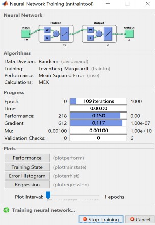
Giao diện của ANN truyền thống trên nền tảng chương trình MATLAB

ANNPSO

%% Empty space clc

clear

rng default tic;

%% Read data

% Read the input file

filename ='Case2_Benthuy.xlsx'; sheet_input ='Sheet1'; sheet_output ='Sheet2';

input = xlsread(filename,sheet_input,'A1:Z10000'); target = xlsread(filename,sheet_output,'A1:Z10000'); inputs = awgn(input',100,'measured');

% inputs=input'; targets=target';

% Select number neuron of input, output and hidden layer

number_input=length(inputs(:,1)); number_output=length(targets(:,1)); number_hidden=100;

%% STEP 1: TRAIN DATA WITH ANN

% Chose your train function in ANN trainFcn ='trainlm';

net = feedforwardnet(number_hidden,trainFcn); net = configure(net,inputs,targets);

net = fitnet(number_hidden,trainFcn);

% Close train window net.trainParam.showWindow = 0;

% Setup Division of Data for Training, Validation, Testing net.divideParam.trainRatio = 70/100; net.divideParam.valRatio = 15/100; net.divideParam.testRatio = 15/100;

% Train

[net] = train(net,inputs,targets)

% error NMSE PSO optimized NN outputs=net(inputs); error_1=outputs - targets;

err_1st = mean(error_1.^2)/mean(var(targets',1));%.^ means square.

x=inputs; t = targets; y = net(x);

perf = perform(net,t,y)

% mean is used to calculate mean values. For example. A= [1 2 3 4]

% mean (A)=(1+2+3+4)/4;

%var returns the variance of the elements of A along the first array

%dimension; see equation of var on Mathwork. err_1st=norm(err_1st)

disp (['the differen between output and target is: ' num2str(err_1st)])

% get the normal NN weights and bias weight_bias = getwb(net);

% setting up parameters parameters.MaxIt = 50;

parameters.nPop = 100; parameters.Lower_Boundary = min(weight_bias); parameters.Upper_Boundary = max(weight_bias);

% parameters.Lower_Boundary = -1.5;

% parameters.Upper_Boundary = 1.5; parameters.c1 = 2;

parameters.c2 = 2;

parameters.w = 1;

parameters.w_damp = 0.99; parameters.nn=err_1st;

% Max epoch max_epoch = 1000;

for epoch = 1 : max_epoch

% numWeightElements(nWE)

nWE=number_hidden*number_input+number_output*number_hidden+number_hidden+number_outp ut;

%% STEP 2: TRAIN WITH PSO

% disp('STEP 2: TRAIN WITH PSO')

[FinalCost,FinalPosition,BestCosts] = PSO (parameters,weight_bias,nWE, number_hidden,number_input,number_output,net,inputs,targets);

xo = FinalPosition(1,:); xbest = xo;

ybest = FinalCost;

%% STEP 3: TRAIN NN SECOND TIME disp('STEP 3: TRAIN NN SECOND TIME')

% Setup Division of Data for Training, Validation, Testing net_2nd.divideParam.trainRatio = 70/100; net_2nd.divideParam.valRatio = 15/100; net_2nd.divideParam.testRatio = 15/100;

% Chose your train function in ANN

Xem tất cả 154 trang.

Ngày đăng: 14/07/2022