Bảng 31. Kiểm định Hausman
Coefficients
(b) fe | (B) re | (b-B) Difference | sqrt(diag(V_b-V_B)) S.E. | |
eta | .3706384 | .3902589 | -.0196205 | .0568951 |
roa | 2.299063 | 1.974135 | .3249278 | .0536668 |
lta | -.1344044 | -.1765107 | .0421063 | .0261662 |
gdp | -.9852082 | -.7601545 | -.2250537 | .2374284 |
inf | -.039737 | -.0882755 | .0485385 | .0956143 |
size | .0288494 | .0276139 | .0012355 | .0131028 |
sec | -.5615198 | -.3919349 | -.1695849 | . |
Có thể bạn quan tâm!
-

 Đánh Giá Hiệu Quả Hoạt Động Của Các Ngân Hàng Thương Mại
 -
 Thống Kê Mô Tả Mẫu Nghiên Cứu Bảng 1. Kết Quả Thống Kê Mô Tả Các Biến Trong Mô Hình
 -
 Hoạt động ngân hàng phi truyền thống và hiệu quả ngân hàng - Trường hợp các ngân hàng thương mại niêm yết Việt Nam giai đoạn 2011 - 2019 - 23
Xem toàn bộ 199 trang tài liệu này.
b = consistent under Ho and Ha; obtained from xtreg B = inconsistent under Ha, efficient under Ho; obtained from xtreg
Test: Ho: difference in coefficients not systematic
chi2(7) = (b-B)'[(V_b-V_B)^(-1)](b-B)
= 0.29
Prob>chi2 = 0.9999
(V_b-V_B is not positive definite)
Bảng 32. Kiểm định Breusch and Pagan Lagrangian multiplier
Breusch and Pagan Lagrangian multiplier test for random effects
te[id,t] = Xb + u[id] + e[id,t]
Var
sd = sqrt(Var)
Estimated results:
.0045863 | .0677219 | |
e | .0020524 | .0453036 |
u | .0009527 | .0308659 |
Test: Var(u) = 0
chibar2(01) = 80.78
Prob > chibar2 = 0.0000
Bảng 33. Kiểm định Wooldridge
Wooldridge test for autocorrelation in panel data H0: no first-order autocorrelation
F( 1, 12) = 2.711
Prob > F = 0.1256
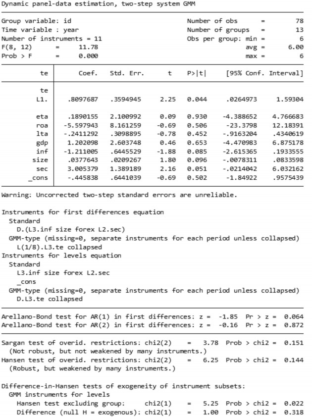
Bảng 34. Kết quả ước lượng mô hình tác động của tỷ lệ thu nhập từ mua bán chứng khoán trên tổng thu nhập (SEC) đến hiệu quả ngân hàng bằng phương pháp SGMM
tổng thu nhập (OTHER) đến hiệu quả ngân hàng bằng phương pháp FEM
Number of obs = | 117 | |
Group variable: id | Number of groups = | 13 |
R-sq: within = 0.1607 | Obs per group: min = | 9 |
between = 0.2601 | avg = | 9.0 |
overall = 0.2109 | max = | 9 |
F(7,97) = | 2.65 | |
corr(u_i, Xb) = 0.1177 | Prob > F = | 0.0149 |
Coef. | Std. Err. t P>|t| [95% Conf. | Interval] | |
eta | -.0041444 | .318114 -0.01 0.990 -.6355126 | .6272239 |
roa | 2.657551 | 1.00546 2.64 0.010 .661992 | 4.65311 |
lta | -.1038434 | .075404 -1.38 0.172 -.2534994 | .0458126 |
gdp | -.8932659 | .628798 -1.42 0.159 -2.141256 | .3547241 |
inf | -.0317707 | .1609205 -0.20 0.844 -.3511534 | .287612 |
size | .0120043 | .0192353 0.62 0.534 -.0261725 | .0501812 |
other | .4533009 | .1670442 2.71 0.008 .1217643 | .7848374 |
_cons | .7956127 | .362283 2.20 0.030 .0765812 | 1.514644 |
sigma_u | .04580431 | ||
sigma_e | .04499346 | ||
rho | .50892961 | (fraction of variance due to u_i) |
F test that all u_i=0: F(12, 97) = 8.80 Prob > F = 0.0000
.
Bảng 36. Kết quả ước lượng mô hình tác động của tỷ lệ thu nhập từ dịch vụ khác trên tổng thu nhập (OTHER) đến hiệu quả ngân hàng bằng phương pháp FEM
Number of obs = | 117 | |
Group variable: id | Number of groups = | 13 |
R-sq: within = 0.1599 | Obs per group: min = | 9 |
between = 0.2712 | avg = | 9.0 |
overall = 0.2175 | max = | 9 |
Wald chi2(7) = | 22.69 | |
corr(u_i, X) = 0 (assumed) | Prob > chi2 = | 0.0019 |
Coef. | Std. Err. z P>|z| [95% Conf. | Interval] | |
eta | .0019204 | .2976689 0.01 0.995 -.5814999 | .5853407 |
roa | 2.663918 | .9279716 2.87 0.004 .8451268 | 4.482709 |
lta | -.1198513 | .070593 -1.70 0.090 -.258211 | .0185083 |
gdp | -.9616096 | .5808864 -1.66 0.098 -2.100126 | .1769068 |
inf | -.0207409 | .1303403 -0.16 0.874 -.2762032 | .2347214 |
size | .0161529 | .0138051 1.17 0.242 -.0109046 | .0432104 |
other | .4615036 | .1609717 2.87 0.004 .146005 | .7770023 |
_cons | .7281435 | .2585681 2.82 0.005 .2213594 | 1.234928 |
sigma_u | .04105015 | ||
sigma_e | .04499346 | ||
rho | .45426688 | (fraction of variance due to u_i) |
.
Coefficients
(b) fe | (B) re | (b-B) Difference | sqrt(diag(V_b-V_B)) S.E. | |
eta | -.0041444 | .0019204 | -.0060648 | .1122041 |
roa | 2.657551 | 2.663918 | -.0063665 | .3870632 |
lta | -.1038434 | -.1198513 | .016008 | .0265027 |
gdp | -.8932659 | -.9616096 | .0683437 | .2407445 |
inf | -.0317707 | -.0207409 | -.0110298 | .0943759 |
size | .0120043 | .0161529 | -.0041485 | .0133947 |
other | .4533009 | .4615036 | -.0082028 | .0446306 |
b = consistent under Ho and Ha; obtained from xtreg B = inconsistent under Ha, efficient under Ho; obtained from xtreg
Test: Ho: difference in coefficients not systematic
chi2(6) = (b-B)'[(V_b-V_B)^(-1)](b-B)
= 7.06
Prob>chi2 = 0.3151
(V_b-V_B is not positive definite)
Bảng 38. Kiểm định Breusch and Pagan Lagrangian multiplier
Breusch and Pagan Lagrangian multiplier test for random effects
te[id,t] = Xb + u[id] + e[id,t]
Var | sd = sqrt(Var) | |
te | .0045863 | .0677219 |
e | .0020244 | .0449935 |
u | .0016851 | .0410501 |
Test: Var(u) = 0
chibar2(01) = 90.15
Prob > chibar2 = 0.0000
Bảng 39. Kiểm định Wooldridge
Wooldridge test for autocorrelation in panel data H0: no first-order autocorrelation
F( 1, 12) = 2.954
Prob > F = 0.1114
tổng thu nhập (OTHER) đến hiệu quả ngân hàng bằng phương pháp SGMM
Dynamic panel-data estimation, two-step system GMM
Number of obs = | 78 | |
Time variable : year | Number of groups = | 13 |
Number of instruments = 11 | Obs per group: min = | 6 |
F(8, 12) = 31.85 | avg = | 6.00 |
Prob > F = 0.000 | max = | 6 |
Coef. | Std. Err. | t | P>|t| | [95% Conf. | Interval] | |
te | ||||||
L1. | -.0622898 | .476442 | -0.13 | 0.898 | -1.100368 | .975788 |
eta | -.4462043 | 2.04453 | -0.22 | 0.831 | -4.900853 | 4.008444 |
roa | -.7590632 | 4.519905 | -0.17 | 0.869 | -10.60709 | 9.088963 |
lta | -.8363086 | .793189 | -1.05 | 0.312 | -2.564519 | .8919017 |
gdp | 3.012647 | 4.241668 | 0.71 | 0.491 | -6.229153 | 12.25445 |
inf | -2.342594 | 1.860461 | -1.26 | 0.232 | -6.396192 | 1.711003 |
size | .0615963 | .0754966 | 0.82 | 0.430 | -.1028965 | .2260892 |
other | 1.489636 | .709911 | 2.10 | 0.058 | -.0571277 | 3.036399 |
_cons | .1821625 | 1.06406 | 0.17 | 0.867 | -2.136226 | 2.500551 |
Warning: Uncorrected two-step standard errors are unreliable.
Instruments for first differences equation Standard
D.(L3.te L.size L2.inf)
GMM-type (missing=0, separate instruments for each period unless collapsed) L(1/8).L2.other collapsed
Instruments for levels equation Standard
L3.te L.size L2.inf
_cons
GMM-type (missing=0, separate instruments for each period unless collapsed) D.L2.other collapsed
Arellano-Bond test for AR(1) in first differences: z = -1.75 Pr > z = 0.080 Arellano-Bond test for AR(2) in first differences: z = 0.09 Pr > z = 0.929
Sargan test of overid. restrictions: chi2(2) = 0.40 Prob > chi2 = 0.820 (Not robust, but not weakened by many instruments.)
Hansen test of overid. restrictions: chi2(2) = 0.47 Prob > chi2 = 0.790 (Robust, but weakened by many instruments.)
Difference-in-Hansen tests of exogeneity of instrument subsets: GMM instruments for levels
Hansen test excluding group: chi2(1) = 0.46 Prob > chi2 = 0.499 Difference (null H = exogenous): chi2(1) = 0.01 Prob > chi2 = 0.908
.