# Output last model: summary(Max_like)
# Mean of AIC, R2adj mean(AIC) mean(R2adj)
# Mean of RMSE, Bias, MAPE%: mean(Bias)
mean(RMSE) mean(MAPE)
# The end
2) Ươc lượng tham số của mô hình theo các nhân tố sinh thái ảnh hưởng
# Erase memory rm(list=ls())
# Clean plot window dev.off()
# Define the working directory
setwd("C:/Users/baohu/OneDrive/PhD Master/PhD Tinh/1. Huong dan Tinh sau cung/Data")
# Import data
t <- read.table("tAll.txt", header=T,sep="t",stringsAsFactors = FALSE)
# Install.packages("ggplot2") library(ggplot2) library(nlme) library(cowplot) library(gridExtra)
# Random Effect Modeling
start <- coefficients(lm(log(AGB)~log(D)+log(H)+log(WD), data=t)) names(start) <- c("a","b","c","d")
start[1]<-exp(start[1])
Max_like <- nlme(AGB~a*D^b*H^c*WD^d, data=t, fixed=a+b+c+d~1, random=a~1, start=start, groups=~Region_simple, weights=varPower(form=~D))
# Output of Model summary( Max_like )
k <- summary(Max_like)$modelStruct$varStruct
# Parameters and random parameters fixef( Max_like )
ranef( Max_like ) coef( Max_like )
coef(summary( Max_like ))
# Standardized Sdi = ai / Si > Si = ai / Sdi > SEi = Si/sqrt(ni)
# Sdi for ai, bi: Sdi = ai, bi / Si
Sdi = ranef( Max_like , standard= TRUE) Sdi
# Standard Deviation: Si = ai, bi / Sdi: Si = ranef( Max_like )/Sdi
Si
# SE for ai, bi: SEi = Si / sqrt(ni)
SEi = Si/sqrt(table(t$ Region_simple ))
SEi table(t$Region_simple )
# Fittied values of the model
t$ Max_like.fit <- fitted.values( Max_like ) t$ Max_like.res <- residuals( Max_like )
t$ Max_like.res.weigh <- residuals( Max_like )/t$D^k
# Plot: Observed/Fitted for Classes p <- ggplot(t)
p <- ggplot(t, aes(y=Max_like.fit, x=AGB , pch= Region_simple, cex = 0.2)) p <- p + geom_abline(intercept = 0, slope = 1, col="black", cex=1.5)
p <- p + geom_point(pch=19,cex=0.2)
p <- p + facet_wrap(~ Region_simple )
p <- p + ylab("AGB ước tính qua mô hình (kg)")+ xlab("AGB quan sát (kg)") + theme_bw()
p <- p + labs(title ="")
p = p + theme(axis.title.y = element_text(size = rel(1.7))) p = p + theme(axis.title.x = element_text(size = rel(1.7))) p <- p + theme(plot.title = element_text(size = rel(1.7))) p = p + theme(axis.text.x = element_text(size=15))
p = p + theme(axis.text.y = element_text(size=15)) p = p + ylim(0,1700)
p = p + xlim(0,1700)
p <- p + theme(legend.position="none") # Delete Legend # p
# The end
ii) Phương pháp xem xét ảnh hưởng tổng hợp các nhân tố sinh thái môi trường rừng lên mô hình sinh khối
Các yếu tố sinh thái môi trường rừng tương tác với nhau và có ảnh hưởng tổng lên quá trình tích lũy sinh khối, carbon cây rừng. Trong trường
hợp này, dạng mô hình sinh khối bao gồm hai thành phần như sau (Lessard và ctv, 2001):
(3.16) |
Có thể bạn quan tâm!
-
 Ảnh Hưởng Của Các Nhân Tố Sinh Thái Môi Trường Rừng, Lâm Phần Đến Mô Hình Ước Tính Agb Cây Rừng Khộp
 -
 Mô Hình Sinh Khối Chung Cho Vùng Nhiệt Đới Hay Cho Từng Vùng Sinh Thái Theo Hệ Thống Phân Loại Thực Vật Ưu Thế Rừng Khộp
 -
 Lựa Chọn Phương Pháp Thẩm Định Sai Số Mô Hình Sinh Khối
 -
 Kết Luận, Tồn Tại Và Kiến Nghị
 -
 Thiết lập và thẩm định chéo hệ thống mô hình ước tính sinh khối trên mặt đất cây rừng khộp ở Việt Nam - 19
 -
 Thiết lập và thẩm định chéo hệ thống mô hình ước tính sinh khối trên mặt đất cây rừng khộp ở Việt Nam - 20
Xem toàn bộ 207 trang tài liệu này.

Trong đó:
- BIOMASS MODEL: Mô hình sinh khối
- AVERGE = ![]() , mô hình sinh khối trung bình được lựa chọn qua thẩm định chéo K-Fold
, mô hình sinh khối trung bình được lựa chọn qua thẩm định chéo K-Fold
- MODIFIER = exp(nhân tố sinh thái, môi trường, lâm phần i – giá trị trung bình của từng nhân tố i), mô hình điều chỉnh giá trị dự đoán sinh khối khi các nhân tố sinh thái, môi trường và lâm phần thay đổi so với trung bình của nó.
Để thiết lập mô hình này, ước lượng mô hình phi tuyến tính có trọng số theo phương pháp Maximum Likelihood (Weighted Non-Linear Fixed Models fit by Maximum Likelihood). Codes chạy R minh họa dưới đây.
Codes chạy trong R để lập mô hình sinh khối xét ảnh hưởng tổng hợp các nhân tố sinh thái môi trường rừng:
AGB = = × exp(nhân tố sinh thái môi trường rừng i – giá trị
trung bình của từng nhân tố i)
theo phương pháp (Weighted Non-linear Fixed Effects fit by Maximum Likelihood) và thẩm định chéo K-Fold (K=10), sau đó sử dụng toàn bộ dữ liệu để ước tính các tham số của mô hình
1) Thiết lập và thẩm định chéo mô hình
# Erase memory rm(list=ls())
# Clean plot window dev.off()
# Define the working directory
setwd("C:/Users/baohu/OneDrive/PhD Master/PhD Tinh/1. Huong dan Tinh sau cung/Data")
# Import data
t <- read.table("tAll.txt", header=T,sep="t",stringsAsFactors = FALSE)
# Install.packages("ggplot2") library(ggplot2) library(nlme) library(cowplot) library(gridExtra)
# K-Fold Cross validation
# Create 10 equally size folds t <- t[sample(nrow(t)),]
folds <- cut(seq(1,nrow(t)),breaks=10,labels=FALSE) AIC = rep(0, 10)
R2adj = rep(0, 10) Bias = rep(0, 10) RMSE = rep(0, 10) MAPE = rep(0, 10)
# Perform 10 fold cross validation: for(i in 1:10){
# Segement the data by fold using the which() function testIndexes <- which(folds==i,arr.ind=TRUE)
n_va <- t[testIndexes, ] t_eq <- t[-testIndexes, ]
# Model = Average * Modifier:
start = c(-2.12, 2.39, 1.10,-0.008, -0.023)
names(start) <- c("a","b","d","b2","b3")
Max_like <- nlme(AGB ~ a*D^b*WD^d* exp( b2* (Rain_annual - 1502) + b3*(BA - 12.62) ), data=cbind(t_eq, g="a"), fixed=a+b+d+b2+b3~1, start=start, groups=~g, weights=varPower(form=~D))
# Estimated and Predicted values:
k <- summary(Max_like)$modelStruct$varStruct[1] t_eq$Max_like.fit <- fitted.values(Max_like) t_eq$Max_like.res <- residuals(Max_like) t_eq$Max_like.res.weigh <- residuals(Max_like)/t_eq$D^k
# Calculationof of AIC, R2 AIC[i] <- AIC(Max_like)
R2 <- 1- sum((t_eq$AGB - t_eq$Max_like.fit)^2)/sum((t_eq$AGB - mean(t_eq$AGB))^2)
R2.adjusted <- 1 - (1-R2)*(length(t_eq$AGB)-1)/(length(t_eq$AGB)-6-1) R2adj[i] <- R2.adjusted
# Prediction of the model for validation
n_va$Pred <- predict(Max_like, newdata=cbind(n_va,g="a"))
# Calculation of RMSE, Bias, MAPE% each time:
Bias[i] = 100*mean((n_va$AGB - n_va$Pred)/n_va$AGB)
RMSE[i] = 100*sqrt(mean(((n_va$AGB - n_va$Pred)/n_va$AGB)^2)) MAPE[i] = 100*mean(abs(n_va$AGB - n_va$Pred)/n_va$AGB)
}
i
# Mean of AIC, R2 adj.: mean(AIC) mean(R2adj)
# Mean of RMSE, Bias, MAPE%: mean(Bias)
mean(RMSE) mean(MAPE)
# Output of model: summary(Max_like)
2) Ước lượng các tham số mô hình với toàn bộ dữ liệu, vẽ đồ thị
# Erase memory rm(list=ls())
# Clean plot window dev.off()
# Define the working directory
setwd("C:/Users/baohu/OneDrive/PhD Master/PhD Tinh/1. Huong dan Tinh sau cung/Data")
# Import data
t_eq <- read.table("tAll.txt", header=T,sep="t",stringsAsFactors = FALSE)
# Install.packages("ggplot2") library(ggplot2) library(nlme) library(cowplot) library(gridExtra)
# Modeling
start = c(-2.12, 2.39, 1.10,-0.008, -0.023)
names(start) <- c("a","b", "d","b2","b3")
Max_like <- nlme(AGB ~ a*D^b*WD^d* exp( b2* (Rain_annual - 1502) + b3*(BA - 12.62) ), data=cbind(t_eq, g="a"), fixed=a+b+d+b2+b3~1, start=start, groups=~g, weights=varPower(form=~D))
# Estimated and Predicted values:
k <- summary(Max_like)$modelStruct$varStruct[1] t_eq$Max_like.fit <- fitted.values(Max_like) t_eq$Max_like.res <- residuals(Max_like) t_eq$Max_like.res.weigh <- residuals(Max_like)/t_eq$D^k
# Output of model: summary(Max_like)
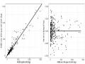
# Plot of Observed/Fitted p1 <- ggplot(t_eq)
p1 <- p1 + geom_point(aes(y=Max_like.fit, x=AGB), cex = 2)
p1 <- p1 + geom_abline(intercept = 0, slope = 1, col="black", cex=1.5)
p1 <- p1 + xlab("AGB quan sát (kg)") + ylab("AGB ước tính qua mô hình (kg)") + theme_bw()
p1 <- p1 + labs(title ="")
p1 = p1 + theme(axis.title.y = element_text(size = rel(1.7))) p1 = p1 + theme(axis.title.x = element_text(size = rel(1.7))) p1 <- p1 + theme(plot.title = element_text(size = rel(1.7))) p1 = p1 + theme(axis.text.x = element_text(size=15))
p1 = p1 + theme(axis.text.y = element_text(size=15)) p1 = p1 + ylim(0,1500)
p1 = p1 + xlim(0,1500) p1
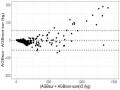
# Plot of Weighted Residuals / Fitted p2 <- ggplot(t_eq)
p2 <- p2 + geom_point(aes(x=Max_like.fit, y=Max_like.res.weigh), cex = 2) p2 <- p2 + geom_line(cex = 1.5, aes(x=Max_like.fit, y=0))
p2 <- p2 + xlab("AGB ước tính qua mô hình (kg)") + ylab("Sai số cso trọng số (kg)") + theme_bw()
p2 <- p2 + labs(title ="")
p2 = p2 + theme(axis.title.y = element_text(size = rel(1.5))) p2 = p2 + theme(axis.title.x = element_text(size = rel(1.5))) p2 <- p2 + theme(plot.title = element_text(size = rel(1.7))) p2 = p2 + theme(axis.text.x = element_text(size=15))
p2 = p2 + theme(axis.text.y = element_text(size=15)) p2 = p2 + ylim(-0.05, 0.05)
p2 = p2 + xlim(0,1500) p2
plot_grid(p1, p2, ncol = 2)
# The end
Sử dụng mô hình dưới đây để ước tính AGB chung cho các loài cây rừng khộp trong đó có sự tham gia điều chỉnh để tăng độ tin cậy ước tính AGB của hai nhân tố sinh thái môi trường rừng là lượng mưa trung bình năm (P, mm/năm) và tổng tiết diện ngang lâm phần (BA, m2/ha)
(3.17) |
3.6.1.8 Kỹ thuật thiết lập đồng thời hệ thống mô hình sinh khối cây rừng theo SUR
Kết quả nghiên cứu đã cho thấy thiết lập hệ thống đồng thời các mô hình sinh khối bộ phận Bst, Bbr, Ble, Bba và AGB theo phương pháp Seemingly Unrelated Regression – SUR đã xem xét mối quan hệ qua lại giữa các thành phần sinh khối cây rừng, do đó đã cải thiện độ tin cậy của ước lượng tổng sinh khối cây trên mặt đất AGB so với phương pháp thiết lập rời rạc, độc lập các mô hình sinh khối bộ phận và tổng AGB.
Sử dụng hệ thống mô hình sau đây để ước tính đồng thời sinh khối cây rừng khộp theo SUR và theo hệ thống phân loại thực vật:
Đối với chung các loài và họ dầu chiếm ưu thế Dipterocarpaceae:
(3.18) |
Đối với chi thực vật ưu thế Dipterocarpus và Shorea:
(3.19) |
Các tham số của hệ thống các mô hình này được trình bày trong Bảng 3.7 Sau đây là codes để lập để thực hiện hệ thống mô hình này trong SAS
Codes để thiết lập đồng thời hệ thống mô hình sinh khối theo SUR và thẩm định chéo K-Fold chạy trong phần mềm SAS
Hệ thống mô hình chung các loài rừng khộp:
AGB = f(Bst + Bbr + Ble +Bba) = a1×Db11×Hb12×WDb13 + a2×Db21 + a3×Db31 + a4×Db41
1) Thiết lập và thẩm định cheo hệ thống mô hình theo SUR dm'log;clear;output;clear';
options pageno=1 nodate nocenter;
/* Create a path to the folder to get input file and write the output to */
%let infile_path = C:UsersbaohuOneDrive1 - Article Dip ForestSAS Scripts for SUR;
%let outfile_path = C:UsersbaohuOneDrive1 - Article Dip ForestSAS Scripts for SUR;
/* Ensure no dataset exists globaly with name we will append TBwts results to */ proc datasets library = work nodetails nolist;
delete B_AGB; run;
quit;
/* Code to load 10 random datasets for DF and EBLF -- datasets generated from script Generate_Random_200_datasets */
data B;
infile "&infile_path.Mix2.csv" dlm=',' firstobs=2 dsd truncover;
input Selected Plot_ID$ ID$ Tree_ID$ FT$ D H WD Bst Bbr Ble Bba AGB D2H D2HWD simNum;
keep Selected D H WD Bst Bbr Ble Bba AGB D2H D2HWD simNum; run;
/* Repeat model fitting and validation statistic calculation 200 times */
%macro runit_var1(eq_num=);
/* Step 1: Subset testing (validation) and training data (model fitting) */ data B_train; set B;
if Selected = 1; run;
data B_test; set B; if Selected = 0; run;
/* Step 2: Fit sur weighted nls models: proc model data=B_train NOPRINT; by simNum;
parms a1=0.032 b11=2.305 b12=0.506 b13=0.796 a2=0.007 b21=2.846
a3=0.019 b31=1.884 a4=0.039 b41=2.216;
Bst = a1*(D**b11)*(H**b12)*(WD**b13); h.Bst = 1/D;
Bbr = a2*(D**b21); h.Bbr = 1/D**-1; Ble = a3*(D**b31); h.Ble = 1/D**2; Bba = a4*(D**b41); h.Bba = 1/D**-2;
AGB = a1*(D**b11)*(H**b12)*(WD**b13) + a2*(D**b21) + a3*(D**b31) + a4*(D**b41);