Durbin-Watson statistic = 0.711779
Lag 1 residual autocorrelation = 0.613465
Residual Analysis
Estimation | Validation | |
n | 100 | |
MSE | 129.862 | |
MAE | 9.7617 | |
MAPE | 9.26129 | |
ME | -0.717794 | |
MPE | -5.01688 |
Có thể bạn quan tâm!
-

 Djiko Soetrisno And Mahyuddin M. D. (1994), “Effect Of Graizing Systems On Reproductive Performance And The Net Return Of Milk Yielded By Shiwal – Friesian (Fs) Cows”, Proceeding Of The 7Th
 -
 Safi Jahanshahi A., Vaez Torshizi R., Kashan N. E. J. And Sayyad Nejad M. B. (2002), “Genetic Parameters For Milk Production Traits Of Iran Holsteins”, Proc. 7Th World Congress On Genetics
 -
 Nghiên cứu khả năng sinh trưởng, sinh sản, năng suất và chất lượng sữa của bò cái holstein friesian HF thuần, các thế hệ lai F1, F2 và F3 giữa HF và lai sind nuôi tại tỉnh Lâm Đồng - 22
Xem toàn bộ 186 trang tài liệu này.
The StatAdvisor
The output shows the results of fitting a nonlinear regression model to describe the relationship between KLF2NTN and 1 independent variables. The equation of the fitted model is
KLF2NTN = 468.184*EXP(-2.37464*EXP(-0.107303*TTNTN))
In performing the fit, the estimation process terminated successully after 7 iterations, at which point the residual sum of squares appeared to approach a minimum.
The R-Squared statistic indicates that the model as fitted explains 99.2372% of the variability in KLF2NTN. The adjusted R-Squared statistic, which is more suitable for comparing models with different numbers of independent variables, is 99.2219%. The standard error of the estimate shows the standard deviation of the residuals to be 11.3957. This value can be used to construct prediction limits for new observations by selecting the Forecasts option from the text menu. The mean absolute error (MAE) of 9.7617 is the average value of the residuals. The Durbin-Watson (DW) statistic tests the residuals to determine if there is any significant correlation based on the order in which they occur in your data file.
The output also shows aymptotic 95.0% confidence intervals for each of the unknown parameters. These intervals are approximate and most accurate for large sample sizes. You can determine whether or not an estimate is statistically significant by examining each interval to see whether it contains the value 0. Intervals covering 0 correspond to coefficients which may well be removed form the model without hurting the fit substantially.
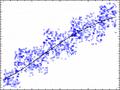
Plot of Fitted Model
500
450
K h o i l u o n g b o F 2 ( k g )
400
350
300
250
200
150
100
50
0
0 6 12 18 24
Thang tuoi
Nonlinear Regression - KLF3NTN
Dependent variable: KLF3NTN Independent variables: TTNTN
Function to be estimated: M*EXP(-A*EXP(-B*TTNTN)) Estimation method: Marquardt
Estimation stopped due to convergence of parameter estimates. Number of iterations: 7
Number of function calls: 31
Estimation Results
Asymptotic | 95.0% | |||
Asymptotic | Confidence | Interval | ||
Parameter | Estimate | Standard Error | Lower | Upper |
M | 490.214 | 8.3501 | 473.801 | 506.946 |
A | 2.37103 | 0.040621 | 2.29041 | 2.45165 |
B | 0.107915 | 0.00355836 | 0.102852 | 0.116977 |
Analysis of Variance
Sum of Squares | Df | Mean Square | |
Model | 7.73198E6 | 3 | 2.57733E6 |
Residual | 13610.8 | 97 | 140.317 |
Total | 7.74559E6 | 100 | |
Total (Corr.) | 1.86283E6 | 99 |
R-Squared = 99.3094 percent
R-Squared (adjusted for d.f.) = 99.2143 percent Standard Error of Est. = 11.8455
Mean absolute error = 10.3627 Durbin-Watson statistic = 0.612331
Lag 1 residual autocorrelation = 0.684735
Residual Analysis
Estimation | Validation | |
n | 100 | |
MSE | 140.317 | |
MAE | 10.3627 | |
MAPE | 10.4534 | |
ME | -0.855128 | |
MPE | -5.99548 |
The StatAdvisor
The output shows the results of fitting a nonlinear regression model to describe the relationship between KLF3NTN and 1 independent variables. The equation of the fitted model is
KLF3NTN = 490.214*EXP(-2.37103*EXP(-0.107915*TTNTN))
In performing the fit, the estimation process terminated successully after 7 iterations, at which point the residual sum of squares appeared to approach a minimum.
The R-Squared statistic indicates that the model as fitted explains 99.3094% of the variability in KLF3NTN. The adjusted R-Squared statistic, which is more suitable for comparing models with different numbers of independent variables, is 99.2143%. The standard error of the estimate shows the standard deviation of the residuals to be 11.8455. This value can be used to construct prediction limits for new observations by selecting the Forecasts option from the text menu. The mean absolute error (MAE) of 10.3627 is the average value of the residuals. The Durbin-Watson (DW) statistic tests the residuals to determine if there is any significant correlation based on the order in which they occur in your data file.
The output also shows aymptotic 95.0% confidence intervals for each of the unknown parameters. These intervals are approximate and most accurate for large sample sizes. You can determine whether or not an estimate is statistically significant by examining each interval to see whether it contains the value 0. Intervals covering 0 correspond to coefficients which may well be removed form the model without hurting the fit substantially.
Plot of Fitted Model
500
450
K h o i l u o n g b o F 3 ( k g )
400
350
300
250
200
150
100
50
0
0 6 12 18 24
Thang tuoi
Nonlinear Regression - KLHFNTN
Dependent variable: KLHFNTN Independent variables: TTNTN
Function to be estimated: M*EXP(-A*EXP(-B*TTNTN)) Estimation method: Marquardt
Estimation stopped due to convergence of residual sum of squares. Number of iterations: 7
Number of function calls: 32
Estimation Results
Asymptotic | 95.0% | |||
Asymptotic | Confidence | Interval | ||
Parameter | Estimate | Standard Error | Lower | Upper |
M | 522.868 | 8.78139 | 505.71 | 540.607 |
A | 2.41096 | 0.0410924 | 2.32941 | 2.49252 |
B | 0.109181 | 0.00350163 | 0.103231 | 0.117131 |
Analysis of Variance
Sum of Squares | Df | Mean Square | |
Model | 8.71709E6 | 3 | 2.9057E6 |
Residual | 14864.8 | 97 | 153.246 |
Total | 8.73195E6 | 100 | |
Total (Corr.) | 2.1363E6 | 99 |
R-Squared = 99.3542 percent
R-Squared (adjusted for d.f.) = 99.2698 percent Standard Error of Est. = 12.3792
Mean absolute error = 10.8623
Durbin-Watson statistic = 0.512386
Lag 1 residual autocorrelation = 0.733998
Residual Analysis
Estimation | Validation | |
n | 100 | |
MSE | 153.246 | |
MAE | 10.8623 | |
MAPE | 11.0878 | |
ME | -0.975136 | |
MPE | -6.6848 |
The StatAdvisor
The output shows the results of fitting a nonlinear regression model to describe the relationship between KLHFNTD and 1 independent variables. The equation of the fitted model is
KLHFNTN = 522.868*EXP(-2.41096*EXP(-0.10981*TTNTN))
In performing the fit, the estimation process terminated successully after 7 iterations, at which point the estimated coefficients appeared to converge to the current estimates.
The R-Squared statistic indicates that the model as fitted explains 99.3542% of the variability in KLHFNTN. The adjusted R-Squared statistic, which is more suitable for comparing models with different numbers of independent variables, is 99.2698%. The standard error of the estimate shows the standard deviation of the residuals to be 12.3792. This value can be used to construct prediction limits for new observations by selecting the Forecasts option from the text menu. The mean absolute error (MAE) of 10.8623 is the average value of the residuals. The Durbin-Watson (DW) statistic tests the residuals to determine if there is any significant correlation based on the order in which they occur in your data file.
The output also shows aymptotic 95.0% confidence intervals for each of the unknown parameters. These intervals are approximate and most accurate for large sample sizes. You can determine whether or not an estimate is statistically significant by examining each interval to see whether it contains the value 0. Intervals covering 0 correspond to coefficients which may well be removed form the model without hurting the fit substantially.
Plot of Fitted Model
500
450
K h o i l u o n g b o H F ( k g )
400
350
300
250
200
150
100
50
0
0 6 12 18 24
Thang tuoi
5. MỘT SỐ HÌNH ẢNH
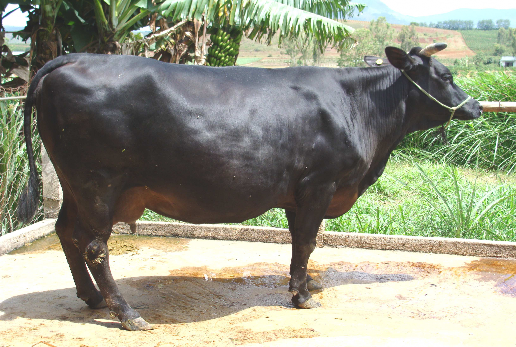
Hình 3. Bò cái F1
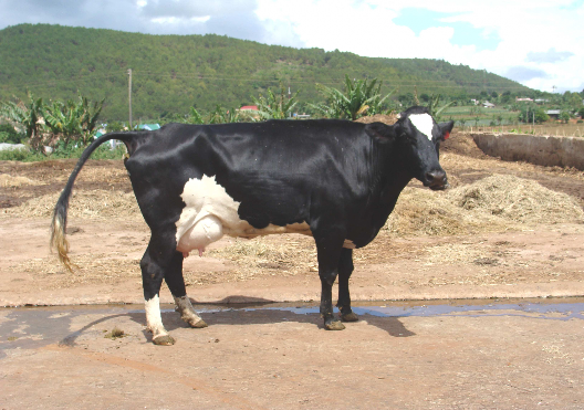
Hình 4. Bò cái F2
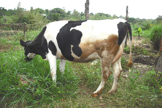
Hình 5. Bò cái F3
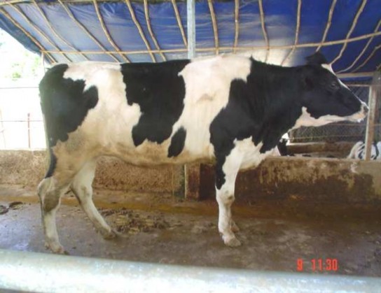
Hình 6. Bò cái HF