Lexicalization Probabilistic Context-Free Grammar

The above problem is solved by the Inside – Outside Algorithm proposed by Baker in 1979 for context-free grammar [81]. This is essentially a variant of the forward – backward algorithm of the hidden Markov model (Hidden Markov Model – HMM). The algorithm allows to calculate the inner and outer probabilities for the input sentence S recursively.

The hidden Markov model, introduced by Manning and Schütze [87], is concerned with the sequence of observations O1,…, Om produced by the laws Ni → NjN k and Ni → wj . Where Oi , i = 1, m are actually the terminating symbols (from) w1,…, wm of the input string.

According to the HMM model, the parameter matrix of the probability context-free grammar is α[i, j, k] and β[i, r] with:

α [i, j, k] = Pr ( Ni → NjNk | G )

β [i, r] = Pr ( Ni→ r | G )

To be able to construct the above parameter matrix, the context-free grammar is assumed to be in Chomsky normal form. This does not reduce the generality of the model, because according to [63], any context-free grammar can be converted to Chomsky normal form. The following constraint is required for the parameters:

∑ α 8i, j, k; + ∑> β 8i, r; = 1 for all i.

This constraint (regarding the i-th non-terminating notation in the grammar) shows that every productive applicability where the left-hand side is the i-th non-terminated symbol can produce only or two non-terminating symbols. or a terminator (due to the grammar in Chomsky normal form).

Maybe you are interested!

Here is the notation convention according to [87]:

The non-terminating symbol set of the grammar is denoted by { N1 ,…, Nn }. The first symbol is N1 .
The terminating symbol set of the grammar is {w1 , …, w V }.
Sentences analyzed w1… wm.
wpq is the part of the sentence that needs to be analyzed from the pth word to the qth word.
NBC ? is a non-terminating symbol Nj that produces a sequence of words at positions from p to q in the sentence.
αj(p, q) is the outer probability.
βj(p, q) is the inner probability.

The probability in βj (p, q) is the probability that the jth non-terminating symbol (Nj ) produces the observation (sequence of words) wp,… .wq. Formally,

βj ( p, q ) = Pr ( wpq | NBC ? , G )

Outer probability αj (p, q) is the probability that starting from the initial symbol N1 produces the non-terminating symbol NBC ? and the words of the input string are outside wp,… , wq. Formally, we have:

αj ( p, q ) = Pr ( w1(p-1), NBC ? , w(q+1)m | G )

The inner and outer probabilities are the basis for building algorithms related to two main problems in parsing probabilistic models, which are:

1. Recognition: Calculate the probability that the first symbol N1 generates the sequence of observations O in the grammar G. Thus, with the algorithm in (Inside Algorithm), the probability that a sentence has m from w1.. The correct wm (produced by the G grammar) is:

Pr ( w1m | G ) = Pr ( N1 ∗ ⇒ w1m | G ) = β1 ( 1, m )

The said probability is the correct probability of the sentence, i.e. the sum of the probabilities of the analyses. To solve the ambiguity problem, it is necessary to find the analysis with the largest probability among the analyses. This problem is solved by the Viterbi type algorithm in the HMM model. Similar to the internal probability algorithm, but this algorithm finds the maximum value instead of the sum. In [87], the whole Viterbi-type algorithm is presented to find the best syntax tree for the sentence w1… .wm.

2. Training: After finding the best parser for the input sentence, the parser needs to continue with the training phase. The training problem can be described as follows: redefine the probability of the rule set in the grammar G given the training sequence of sentences s1, s2,…, sn. The problem of training for a probabilistic context-free grammar was presented in [87].

According to [70], a probabilistic context-free grammar has the following disadvantages:

It is not possible to model the dependencies between structures on the syntax tree because the probabilities of each rule are calculated completely independent of each other.
Lack of lexical information: Syntax information may be related to particular words, but the context-free model is not descriptive. This leads to ambiguity in coordination, subcategory, and prepositional use.

1.1.3. lexicalization probabilistic context-free grammar

The lexicalized probabilistic context-free grammar not only shows the structure of phrases but also shows the relationship between words. In a Lexicalized Probabilistic Context Free Grammar, each non-terminating symbol is written as A(x), x = (w, t) where A is the label of the structure. The number of non-terminating symbols will increase dramatically, at most until |ν| × |τ| times, |ν| is the number of words in the vocabulary and |τ| is the number of type words of the language

The law of a context-free grammar of lexicalization probability takes the form:

1. Internal law:

P(h) → Ln(ln)…L1(l1) H(h) R1(r1) … Rm(rm) (1.1)

In which, h is the pair of words/labels of the type. H is the principal child of the rule, will inherit the word/label pair from the parent node’s type P. The component Ln(ln) … L1(l1) modifies the H on the left and the element R1(r1).. Rm(rm) modifies the H on the right (n or m can be zero). The left and right ranges are extended by the STOP notation. So Ln+1 = Rm+1 = STOP

2. Vocabulary law:

P(h) → w, P is a type label word, h is a (w, t) pair (1.2)

Figure 1.3. The following illustrates a lexicalized probabilistic context-free grammar [43].

When calculating the probability for each production, adding lexical information makes the denominator extremely large, the probability is almost zero.

To avoid the number of parameters being too large, in the model given by Collins [43], the probability of the intrinsic law is calculated based on the probability series law.

The probability of generating a modifier can depend on any function of the previous modifiers, the domain of the central word or the central word. Therefore, distance is added [43] to the assumption of independence of modifiers.

This model has also been used by Le Thanh Huong group [22] to build a Vietnamese parser with the comment “In Vietnamese, the boundary components of languages depend more on the component next to it than on the term’s boundary components. depends on the central component”. In [22], a formula for calculating the probability of a rule for boundary components has no appearance of the distance and a formula for calculating the probability of a rule with added probability values connecting words on either side of the component. main of the right-hand side.

Judiciary (production)

Intrinsic Laws

TOP → S(bought, VBD)

S(bought, VBD → NP(week, NN) NP(IBM, NNP) VP(bought, VBD)

NP(week, NN → JJ(Last, JJ) NN(week,NN)

NP(IBM, NNP) → NNP(IBM, NNP)

VP(bought, VBD) → VBD(bought,VBD) NP(Lotus,NNP)

NP(Lotus, NNP) → NNP(Lotus, NNP)

Vocabulary rules

JJ(last, JJ) → last

NP(week, NN) → week

NNP(IBM, NNP) → IBM

VBD(bought,VBD) → bought

NP(Lotus, NNP) → Lotus

Structural tree for sentences ”Last week IBM bought Lotus”

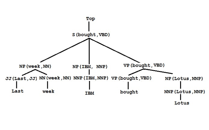
Figure 1.3. Probabilistic context-free grammar and sentence structure tree “Last week IBM bought Lotus”

1.1.4. Tree connection grammar

With the advent of treebanks, rewrite operations on the grammar can no longer take place on strings, but on the structure tree.

The base element of the Tree Adjoining Grammar (TAG) is the basic tree [69]. The underlying trees are joined together through two rewrites, combine and replace. The intermediate trees that are generated when substitutions and joins are applied are called parse trees.

A full parse tree is an parse tree in which every leaf node has a label as the termination symbol. The parsing for a sentence can be understood as: starting from a basic tree whose root is the axiom, find a complete parse tree whose leaf nodes correspond to the sequence of words in the sentence.

The TAG grammar is lexicalized to become LTAG (Lexicalized Tree Adjoining Grammar). This is also a completely lexicalized grammar. Every elementary tree has at least one leaf node associated with a lexical unit called an anchor word. In addition, the grammar also satisfies the following conditions:

Each LTAG initialization tree represents the components of an anchor word (component modifiers for the anchor word).
Basic trees are minimal: the initialization tree must have the word anchor that is the center word of a principal element in the sentence and contain all the mandatory opposites of the word anchor [20].

Date published: 01/11/2021