Credit market share (%)
State-owned commercial banks Joint-stock commercial banks
Foreign banks
Other
2007
2008
2009
2010
2011
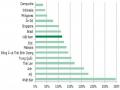
Meanwhile, the level of market concentration on credit shows that there is a group monopoly of state-owned commercial banks. If the capital mobilization market share in the period 2007 - 2011 had a large shift from state-owned commercial banks to joint stock commercial banks, the credit market share did not change significantly between the two banks. This banking sector (Figure A.3 shows that the credit market share of state-owned commercial banks only decreased slightly from 59.3% to 51.3% in the period 2007 - 2011), clearly demonstrating the competitive advantage between the two banks. block. State-owned commercial banks hold a high credit market share thanks to their wide networks covering key economic provinces. Lending to key economic projects of the state or having close relationships with economic groups are the factors that determine the difference in credit market share. Joint-stock commercial banks do not have such advantages, so credit is concentrated on individual customers and small and medium-sized enterprises, so accelerating the expansion of credit market share will be difficult. The high degree of concentration indicates the dominance of state-owned commercial banks and is a factor undermining the importance of the channel.bank loans in Vietnam.
9.2 | 11 | 9.1 | 9 | 8.6 | ||||||||||
27.7 | 26.5 | 32 | 35.1 | 35.5 | ||||||||||
59.3 | 58.1 | |||||||||||||
54.1 | 51.4 | 51.3 | ||||||||||||
Maybe you are interested!
-

 Bank lending channel and monetary policy transmission in Vietnam - 4
 -
 Macroeconomic Impact Of Bank Lending Channel
 -
 Bank lending channel and monetary policy transmission in Vietnam - 6
 -
 Bank lending channel and monetary policy transmission in Vietnam - 8

Figure A.3. Credit market share of Vietnamese banks in the period 2007 - 2011
Source: VNEconomy
In summary, the evidence describing the strength of the bank lending channel in Vietnam is mixed. Factors such as a high degree of market concentration in credit, or a high degree of state involvement in the banking sector, suggest that the lending channel will be weak. On the other hand, factors such as the high level of competition for capital mobilization, the low level of foreign ownership, or the high degree of banking dependence of domestic organizations and individuals, are supportive factors for Vietnam's economic growth. existence of a bank lending channel. Furthermore, the banking industry in Vietnam is quite diversified, and there are a large number of small banks with weak balance sheet structures, and therefore different ratios of size, liquidity, and capitalization. significantly different from the banking industry average. Therefore, to draw conclusions about the role of the banking industry in Vietnam in monetary policy transmission, we need to do some formal empirical testing.
APPENDIX B. ESTIMATE RESULTS
B.1. Model estimation results (4.1) using scale characteristics
Dynamic panel-data estimation, one-step system GMM
Group variable: crossid | Number of obs | = | 265 |
Time variable : timeid | Number of groups | = | 30 |
Number of instruments = 38 | Obs per group: min | = | 7 |
F(10, 29) = 645.84 | avg | = | 8.83 |
Prob > F = 0.000 max = 9
lnloan | Coef. | Robust Std. Err. | t | P>|t| | [95% Conf. | Interval] |
lnloan | ||||||
L1. | .5500024 | .079507 | 6.92 | 0.000 | .3873923 | .7126125 |
rate | ||||||
--. | -.1210267 | .0313966 | -3.85 | 0.001 | -.1852401 | -.0568133 |
L1. | .0383065 | .0375161 | 1.02 | 0.316 | -.0384225 | .1150355 |
gdp | ||||||
--. | .2361301 | .0969511 | 2.44 | 0.021 | .0378428 | .4344174 |
L1. | -.3675458 | .0533824 | -6.89 | 0.000 | -.4767252 | -.2583665 |
CPI | ||||||
--. | .0803953 | .0168616 | 4.77 | 0.000 | .0459094 | .1148812 |
L1. | .0032086 | .0251175 | 0.13 | 0.899 | -.0481624 | .0545797 |
size | ||||||
L1. | .3157022 | .0680192 | 4.64 | 0.000 | .1765874 | .4548171 |
size1rate | .006341 | .0027095 | 2.34 | 0.026 | .0007994 | .0118826 |
size1rate1 | .0015955 | .0028599 | 0.56 | 0.581 | -.0042536 | .0074447 |
_cons | 8.500045 | 1.898784 | 4.48 | 0.000 | 4.616596 | 12.38349 |
Instruments for first differences equation Standard
D.(rate L.rate gdp L.gdp cpi L.cpi)
GMM-type (missing=0, separate instruments for each period unless collapsed) L2.(L.lnloan L.size size1rate size1rate1)
Instruments for levels equation Standard
rate L.rate gdp L.gdp cpi L.cpi
_cons
GMM-type (missing=0, separate instruments for each period unless collapsed) DL.(L.lnloan L.size size1rate size1rate1)
Arellano-Bond test for AR(1) in first differences: z = -3.60 Pr > z = 0.000 Arellano-Bond test for AR(2) in first differences: z = -0.41 Pr > z = 0.683
Sargan test of overid. restrictions: chi2(27) = 154.75 Prob > chi2 = 0.000 (Not robust, but not weakened by many instruments.)
Hansen test of overid. restrictions: chi2(27) = 22.61 Prob > chi2 = 0.706 (Robust, but weakened by many instruments.)
Difference-in-Hansen tests of exogeneity of instrument subsets:
Hansen test excluding group: chi2(10) | = | 20.37 | Prob | > | chi2 | = | 0.026 |
Difference (null H = exogenous): chi2(17) | = | 2.24 | Prob | > | chi2 | = | 1,000 yen |
Hansen test excluding group: chi2(21) | = | 19.95 | Prob | > | chi2 | = | 0.524 |
Difference (null H = exogenous): chi2(6) | = | 2.65 | Prob | > | chi2 | = | 0.851 |
GMM instruments for levels
iv(rate L.rate gdp L.gdp cpi L.cpi)
B.2. Model estimation results (4.1) using liquidity characteristics
Dynamic panel-data estimation, one-step system GMM
Group variable: crossid | Number of obs | = | 265 |
Time variable : timeid | Number of groups | = | 30 |
Number of instruments = 38 | Obs per group: min | = | 7 |
F(10, 29) = 534.18 | avg | = | 8.83 |
Prob > F = 0.000 max = 9
lnloan | Coef. | Robust Std. Err. | t | P>|t| | [95% Conf. | Interval] |
lnloan | ||||||
L1. | .8901591 | .0299489 | 29.72 | 0.000 | .8289068 | .9514115 |
rate | ||||||
--. | -.0071375 | .0185304 | -0.39 | 0.703 | -.0450365 | .0307614 |
L1. | -.1141464 | .0234951 | -4.86 | 0.000 | -.1621992 | -.0660936 |
gdp | ||||||
--. | .5937123 | .084833 | 7.00 | 0.000 | .4202094 | .7672152 |
L1. | -.212927 | .0428574 | -4.97 | 0.000 | -.3005803 | -.1252737 |
CPI | ||||||
--. | .0226894 | .0123305 | 1.84 | 0.076 | -.0025293 | .0479082 |
L1. | .1016865 | .0182143 | 5.58 | 0.000 | .064434 | .1389389 |
liq | ||||||
L1. | .3688341 | .6786717 | 0.54 | 0.591 | -1.019205 | 1.756874 |
liq1rate | -.0014729 | .0516665 | -0.03 | 0.977 | -.1071427 | .1041969 |
liq1rate1 | -.0015223 | .0341104 | -0.04 | 0.965 | -.0712859 | .0682413 |
_cons | -.3101139 | .686045 | -0.45 | 0.655 | -1.713234 | 1.093006 |
Instruments for first differences equation Standard
D.(rate L.rate gdp L.gdp cpi L.cpi)
GMM-type (missing=0, separate instruments for each period unless collapsed) L2.(L.lnloan L.liq liq1rate liq1rate1)
Instruments for levels equation Standard
rate L.rate gdp L.gdp cpi L.cpi
_cons
GMM-type (missing=0, separate instruments for each period unless collapsed) DL.(L.lnloan L.liq liq1rate liq1rate1)
Arellano-Bond test for AR(1) in first differences: z = -3.44 Pr > z = 0.001 Arellano-Bond test for AR(2) in first differences: z = -1.26 Pr > z = 0.206
Sargan test of overid. restrictions: chi2(27) = 105.87 Prob > chi2 = 0.000 (Not robust, but not weakened by many instruments.)
Hansen test of overid. restrictions: chi2(27) = 27.02 Prob > chi2 = 0.463 (Robust, but weakened by many instruments.)
Difference-in-Hansen tests of exogeneity of instrument subsets:
Hansen test excluding group: chi2(10) | = | 15.27 | Prob | > | chi2 | = | 0.123 |
Difference (null H = exogenous): chi2(17) | = | 11.75 | Prob | > | chi2 | = | 0.815 |
Hansen test excluding group: chi2(21) | = | 22.35 | Prob | > | chi2 | = | 0.380 |
Difference (null H = exogenous): chi2(6) | = | 4.67 | Prob | > | chi2 | = | 0.587 |
GMM instruments for levels
iv(rate L.rate gdp L.gdp cpi L.cpi)
B.3. Model estimation results (4.1) using capitalization characteristics
Dynamic panel-data estimation, one-step system GMM
Group variable: crossid | Number of obs | = | 265 |
Time variable : timeid | Number of groups | = | 30 |
Number of instruments = 38 | Obs per group: min | = | 7 |
F(10, 29) = 559.85 | avg | = | 8.83 |
Prob > F = 0.000 | max | = | 9 |
lnloan | Coef. | Robust Std. Err. | t | P>|t| | [95% Conf. | Interval] |
lnloan | ||||||
L1. | .8812914 | .0472342 | 18.66 | 0.000 | .7846867 | .9778962 |
rate | ||||||
--. | -.0155856 | .0217573 | -0.72 | 0.480 | -.0600842 | .028913 |
L1. | -.1154434 | .0237919 | -4.85 | 0.000 | -.1641032 | -.0667835 |
gdp | ||||||
--. | .6137482 | .0772304 | 7.95 | 0.000 | .4557943 | .7777022 |
L1. | -.2356657 | .0481896 | -4.89 | 0.000 | -.3342245 | -.1371069 |
CPI | ||||||
--. | .030708 | .0134949 | 2.28 | 0.030 | .0031077 | .0583082 |
L1. | .1052771 | .0173324 | 6.07 | 0.000 | .0698284 | .1407259 |
cap | ||||||
L1. | -.3085769 | 1.501278 | -0.21 | 0.839 | -3.379035 | 2.761881 |
cap1rate | .0119564 | .0515935 | 0.23 | 0.818 | -.0935641 | .117477 |
cap1rate1 | -.0021952 | .07092 | -0.03 | 0.976 | -.1472428 | .1428524 |
_cons | -.1752537 | .9951344 | -0.18 | 0.861 | -2.210532 | 1.860025 |
Instruments for first differences equation Standard
D.(rate L.rate gdp L.gdp cpi L.cpi)
GMM-type (missing=0, separate instruments for each period unless collapsed) L2.(L.lnloan L.cap cap1rate cap1rate1)
Instruments for levels equation Standard
rate L.rate gdp L.gdp cpi L.cpi
_cons
GMM-type (missing=0, separate instruments for each period unless collapsed) DL.(L.lnloan L.cap cap1rate cap1rate1)
Arellano-Bond test for AR(1) in first differences: z = -3.52 Pr > z = 0.000 Arellano-Bond test for AR(2) in first differences: z = -1.23 Pr > z = 0.220
Sargan test of overid. restrictions: chi2(27) = 146.83 Prob > chi2 = 0.000 (Not robust, but not weakened by many instruments.)
Hansen test of overid. restrictions: chi2(27) = 22.35 Prob > chi2 = 0.720 (Robust, but weakened by many instruments.)
Difference-in-Hansen tests of exogeneity of instrument subsets:
Hansen test excluding group: chi2(10) | = | 14.84 | Prob | > | chi2 | = | 0.138 |
Difference (null H = exogenous): chi2(17) | = | 7.50 | Prob | > | chi2 | = | 0.976 |
Hansen test excluding group: chi2(21) | = | 20.15 | Prob | > | chi2 | = | 0.512 |
Difference (null H = exogenous): chi2(6) | = | 2.20 | Prob | > | chi2 | = | 0.900 |
GMM instruments for levels
iv(rate L.rate gdp L.gdp cpi L.cpi)
B.4. Model estimation results (4.1) using size and liquidity characteristics
Dynamic panel-data estimation, one-step system GMM
Group variable: crossid | Number of obs | = | 265 |
Time variable : timeid | Number of groups | = | 30 |
Number of instruments = 55 | Obs per group: min | = | 7 |
F(13, 29) = 648.25 | avg | = | 8.83 |
Prob > F = 0.000 | max | = | 9 |
lnloan | Coef. | Robust Std. Err. | t | P>|t| | [95% Conf. | Interval] |
lnloan | ||||||
L1. | .5569479 | .0844174 | 6.60 | 0.000 | .384295 | .7296008 |
rate | ||||||
--. | -.1254419 | .0343049 | -3.66 | 0.001 | -.1956033 | -.0552805 |
L1. | .0355877 | .0415238 | 0.86 | 0.398 | -.049338 | .1205134 |
gdp | ||||||
--. | .2555684 | .0990579 | 2.58 | 0.015 | .0529722 | .4581646 |
L1. | -.3765908 | .0540196 | -6.97 | 0.000 | -.4870733 | -.2661082 |
CPI --. | .085438 | .018637 | 4.58 | 0.000 | .047321 | .1235549 |
L1. | .0070616 | .0273563 | 0.26 | 0.798 | -.0488883 | .0630114 |
size L1. | .3186181 | .0756823 | 4.21 | 0.000 | .1638304 | .4734057 |
size1rate | .0058492 | .0023938 | 2.44 | 0.021 | .0009532 | .0107451 |
size1rate1 | .0013546 | .0029913 | 0.45 | 0.654 | -.0047632 | .0074725 |
liq L1. | -.1588848 | .6483918 | -0.25 | 0.808 | -1.484995 | 1.167225 |
liq1rate | -.0130061 | .0421777 | -0.31 | 0.760 | -.0992693 | .0732571 |
liq1rate1 | -.0086709 | .0290616 | -0.30 | 0.768 | -.0681085 | .05076667 |
_cons | 8.296876 | 1.981204 | 4.19 | 0.000 | 4.24486 | 12,34889 |
Instruments for first differences equation Standard
D.(rate L.rate gdp L.gdp cpi L.cpi)
GMM-type (missing=0, separate instruments for each period unless collapsed) L2.(L.lnloan L.size size1rate size1rate1 L.liq liq1rate liq1rate1)
Instruments for levels equation Standard
rate L.rate gdp L.gdp cpi L.cpi
_cons
GMM-type (missing=0, separate instruments for each period unless collapsed) DL.(L.lnloan L.size size1rate size1rate1 L.liq liq1rate liq1rate1)
Arellano-Bond test for AR(1) in first differences: z = -3.61 Pr > z = 0.000 Arellano-Bond test for AR(2) in first differences: z = -0.64 Pr > z = 0.520
Sargan test of overid. restrictions: chi2(41) = 173.96 Prob > chi2 = 0.000 (Not robust, but not weakened by many instruments.)
Hansen test of overid. restrictions: chi2(41) = 22.02 Prob > chi2 = 0.993 (Robust, but weakened by many instruments.)
Difference-in-Hansen tests of exogeneity of instrument subsets:
Hansen test excluding group: chi2(14) | = | 21.49 | Prob | > | chi2 | = | 0.090 |
Difference (null H = exogenous): chi2(27) | = | 0.53 | Prob | > | chi2 | = | 1,000 yen |
Hansen test excluding group: chi2(35) | = | 20.14 | Prob | > | chi2 | = | 0.979 |
Difference (null H = exogenous): chi2(6) | = | 1.88 | Prob | > | chi2 | = | 0.931 |
GMM instruments for levels
iv(rate L.rate gdp L.gdp cpi L.cpi)
B.5. Model estimation results (4.1) using size and capitalization characteristics
Dynamic panel-data estimation, one-step system GMM
Group variable: crossid | Number of obs | = | 265 |
Time variable : timeid | Number of groups | = | 30 |
Number of instruments = 55 | Obs per group: min | = | 7 |
F(13, 29) = 973.99 | avg | = | 8.83 |
Prob > F = 0.000 | max | = | 9 |
lnloan | Coef. | Robust Std. Err. | t | P>|t| | [95% Conf. | Interval] |
lnloan | ||||||
L1. | .5754071 | .0923473 | 6.23 | 0.000 | .3865358 | .7642785 |
rate | ||||||
--. | -.1171762 | .03586464 | -3.27 | 0.003 | -.1904903 | -.043862 |
L1. | .0517326 | .0527101 | 0.98 | 0.334 | -.0560717 | .1595369 |
gdp | ||||||
--. | .2107098 | .1438594 | 1.46 | 0.154 | -.0835157 | .5049353 |
L1. | -.3390027 | .0515885 | -6.57 | 0.000 | -.4445131 | -.2334923 |
CPI | ||||||
--. | .075852 | .018422 | 4.12 | 0.000 | .0381747 | .1135293 |
L1. | -.0063865 | .03635 | -0.18 | 0.862 | -.0807306 | .0679575 |
size | ||||||
L1. | .3055084 | .1462078 | 2.09 | 0.046 | .0064799 | .604537 |
size1rate | .0134564 | .0056655 | 2.38 | 0.024 | .001869 | .0250437 |
size1rate1 | -.0009326 | .0040038 | -0.23 | 0.817 | -.0091214 | .0072562 |
cap | ||||||
L1. | -.2689005 | 2.120223 | -0.13 | 0.900 | -4.605243 | 4.067443 |
cap1rate | .1943278 | .104508 | 1.86 | 0.073 | -.019415 | .4080707 |
cap1rate1 | -.0345468 | .08700594 | -0.40 | 0.694 | -.2126033 | .1435097 |
_cons | 8.041952 | 2.422732 | 3.32 | 0.002 | 3.086909 | 12,99699 |
Instruments for first differences equation Standard
D.(rate L.rate gdp L.gdp cpi L.cpi)
GMM-type (missing=0, separate instruments for each period unless collapsed) L2.(L.lnloan L.size size1rate size1rate1 L.cap cap1rate cap1rate1)
Instruments for levels equation Standard
rate L.rate gdp L.gdp cpi L.cpi
_cons
GMM-type (missing=0, separate instruments for each period unless collapsed) DL.(L.lnloan L.size size1rate size1rate1 L.cap cap1rate cap1rate1)
Arellano-Bond test for AR(1) in first differences: z = -3.61 Pr > z = 0.000 Arellano-Bond test for AR(2) in first differences: z = -0.68 Pr > z = 0.497
Sargan test of overid. restrictions: chi2(41) = 196.99 Prob > chi2 = 0.000 (Not robust, but not weakened by many instruments.)
Hansen test of overid. restrictions: chi2(41) = 20.49 Prob > chi2 = 0.997 (Robust, but weakened by many instruments.)
Difference-in-Hansen tests of exogeneity of instrument subsets: GMM instruments for levels
Hansen test excluding group: chi2(14) = 13.84 Prob > chi2 = 0.462 Difference (null H = exogenous): chi2(27) = 6.65 Prob > chi2 = 1,000
iv(rate L.rate gdp L.gdp cpi L.cpi)
Hansen test excluding group: chi2(35) = 19.11 Prob > chi2 = 0.987 Difference (null H = exogenous): chi2(6) = 1.38 Prob > chi2 = 0.967
B.6. Model estimation results (4.1) using liquidity and capitalization characteristics
Dynamic panel-data estimation, one-step system GMM
Group variable: crossid | Number of obs | = | 265 |
Time variable : timeid | Number of groups | = | 30 |
Number of instruments = 55 | Obs per group: min | = | 7 |
F(13, 29) = 569.26 | avg | = | 8.83 |
Prob > F = 0.000 max = 9
lnloan | Coef. | Robust Std. Err. | t | P>|t| | [95% Conf. | Interval] |
lnloan | ||||||
L1. | .9200836 | .045702 | 20.13 | 0.000 | .8266126 | 1.013555 |
rate | ||||||
--. | .0010052 | .021956 | 0.05 | 0.964 | -.0438999 | .0459103 |
L1. | -.1221536 | .0220634 | -5.54 | 0.000 | -.1672783 | -.077029 |
gdp | ||||||
--. | .6148317 | .0816434 | 7.53 | 0.000 | .4478522 | .7818112 |
L1. | -.1947507 | .0489473 | -3.98 | 0.000 | -.2948591 | -.0946423 |
CPI | ||||||
--. | .01181704 | .0143775 | 1.26 | 0.216 | -.0112348 | .0475757 |
L1. | .1068964 | .0167063 | 6.40 | 0.000 | .0727283 | .1410646 |
liq | ||||||
L1. | .9285027 | .6717476 | 1.38 | 0.177 | -.4453755 | 2.302381 |
liq1rate | -.0118667 | .0438091 | -0.27 | 0.788 | -.1014665 | .0777733 |
liq1rate1 | -.0430749 | .03364825 | -1.18 | 0.247 | -.11769 | .0315402 |
cap | ||||||
L1. | -.0537768 | 1.705749 | -0.03 | 0.975 | -3.542426 | 3.434872 |
cap1rate | .0216311 | .0650949 | 0.33 | 0.742 | -.1115029 | .1547651 |
cap1rate1 | .0121737 | .0634756 | 0.19 | 0.849 | -.1176484 | .1419958 |
_cons | -1.052049 | .94777637 | -1.11 | 0.276 | -2.990444 | .8863451 |
Instruments for first differences equation Standard
D.(rate L.rate gdp L.gdp cpi L.cpi)
GMM-type (missing=0, separate instruments for each period unless collapsed) L2.(L.lnloan L.liq liq1rate liq1rate1 L.cap cap1rate cap1rate1)
Instruments for levels equation Standard
rate L.rate gdp L.gdp cpi L.cpi
_cons
GMM-type (missing=0, separate instruments for each period unless collapsed) DL.(L.lnloan L.liq liq1rate liq1rate1 L.cap cap1rate cap1rate1)
Arellano-Bond test for AR(1) in first differences: z = -3.48 Pr > z = 0.001 Arellano-Bond test for AR(2) in first differences: z = -0.95 Pr > z = 0.344
Sargan test of overid. restrictions: chi2(41) = 200.86 Prob > chi2 = 0.000 (Not robust, but not weakened by many instruments.)
Hansen test of overid. restrictions: chi2(41) = 21.81 Prob > chi2 = 0.994 (Robust, but weakened by many instruments.)
Difference-in-Hansen tests of exogeneity of instrument subsets:
Hansen test excluding group: chi2(14) | = | 16.85 | Prob | > | chi2 | = | 0.264 |
Difference (null H = exogenous): chi2(27) | = | 4.96 | Prob | > | chi2 | = | 1,000 yen |
Hansen test excluding group: chi2(35) | = | 16.93 | Prob | > | chi2 | = | 0.996 |
Difference (null H = exogenous): chi2(6) | = | 4.88 | Prob | > | chi2 | = | 0.559 |
GMM instruments for levels
iv(rate L.rate gdp L.gdp cpi L.cpi)
B.7. Model estimation results (4.1) using size, liquidity, and capitalization characteristics
Dynamic panel-data estimation, one-step system GMM
Group variable: crossid | Number of obs | = | 265 |
Time variable : timeid | Number of groups | = | 30 |
Number of instruments = 71 | Obs per group: min | = | 7 |
F(16, 29) = 1050.13 | avg | = | 8.83 |
Prob > F = 0.000 | max | = | 9 |
lnloan | Coef. | Robust Std. Err. | t | P>|t| | [95% Conf. | Interval] |
lnloan | ||||||
L1. | .5571485 | .0935599 | 5.95 | 0.000 | .3657971 | .7484999 |
rate | ||||||
--. | -.1285402 | .0382982 | -3.36 | 0.002 | -.2068689 | -.0502116 |
L1. | .0649837 | .0501217 | 1.30 | 0.205 | -.0375266 | .167494 |
gdp | ||||||
--. | .1900537 | .126707 | 1.50 | 0.144 | -.0690913 | .4491986 |
L1. | -.3485914 | .0525653 | -6.63 | 0.000 | -.4560995 | -.2410833 |
CPI | ||||||
--. | .0822325 | .0201086 | 4.09 | 0.000 | .0411059 | .1233592 |
L1. | -.0133686 | .0340265 | -0.39 | 0.697 | -.0829606 | .0562233 |
size | ||||||
L1. | .3203392 | .1357901 | 2.36 | 0.025 | .0426173 | .5980611 |
size1rate | .0138705 | .005192 | 2.67 | 0.012 | .0032517 | .024893 |
size1rate1 | -.0008301 | .0043102 | -0.19 | 0.849 | -.0096454 | .0079853 |
liq | ||||||
L1. | -.0458372 | .6246038 | -0.07 | 0.942 | -1.323295 | 1.231621 |
liq1rate | .0154562 | .0460302 | 0.34 | 0.739 | -.0786862 | .1095986 |
liq1rate1 | -.0399053 | .0322981 | -1.24 | 0.227 | -.1059624 | .0261518 |
cap | ||||||
L1. | -.4207595 | 2.020283 | -0.21 | 0.836 | -4.552702 | 3.711183 |
cap1rate | .2112643 | .0968293 | 2.18 | 0.037 | .0132262 | .4093025 |
cap1rate1 | -.0390466 | .0943169 | -0.41 | 0.682 | -.2319464 | .1538532 |
_cons | 8.516561 | 2.329934 | 3.66 | 0.001 | 3.751311 | 13.28181 |
Instruments for first differences equation Standard
D.(rate L.rate gdp L.gdp cpi L.cpi)
GMM-type (missing=0, separate instruments for each period unless collapsed) L2.(L.lnloan L.size size1rate size1rate1 L.liq liq1rate liq1rate1 L.cap cap1rate cap1rate1)
Instruments for levels equation Standard
rate L.rate gdp L.gdp cpi L.cpi
_cons
GMM-type (missing=0, separate instruments for each period unless collapsed) DL.(L.lnloan L.size size1rate size1rate1 L.liq liq1rate liq1rate1 L.cap cap1rate cap1rate1)
Arellano-Bond test for AR(1) in first differences: z = -3.57 Pr > z = 0.000 Arellano-Bond test for AR(2) in first differences: z = -0.49 Pr > z = 0.624
Sargan test of overid. restrictions: chi2(54) = 207.53 Prob > chi2 = 0.000 (Not robust, but not weakened by many instruments.)
Hansen test of overid. restrictions: chi2(54) = 17.00 Prob > chi2 = 1,000 (Robust, but weakened by many instruments.)
Difference-in-Hansen tests of exogeneity of instrument subsets:
Hansen test excluding group: chi2(18) | = | 16.32 | Prob | > | chi2 | = | 0.570 |
Difference (null H = exogenous): chi2(36) | = | 0.68 | Prob | > | chi2 | = | 1,000 yen |
Hansen test excluding group: chi2(48) | = | 17.08 | Prob | > | chi2 | = | 1,000 yen |
Difference (null H = exogenous): chi2(6) | = | -0.08 | Prob | > | chi2 | = | 1,000 yen |
GMM instruments for levels
iv(rate L.rate gdp L.gdp cpi L.cpi)
B.8. Model estimation results (4.2) using scale characteristics
Dynamic panel-data estimation, one-step system GMM
Group variable: crossid | Number of obs | = | 265 |
Time variable : timeid | Number of groups | = | 30 |
Number of instruments = 40 | Obs per group: min | = | 7 |
F(13, 29) = 545.47 | avg | = | 8.83 |
Prob > F = 0.000 | max | = | 9 |
lnloan | Coef. | Robust Std. Err. | t | P>|t| | [95% Conf. | Interval] |
lnloan | ||||||
L1. | .5737825 | .0708745 | 8.10 | 0.000 | .4288278 | .7187372 |
rate | ||||||
--. | -.114008 | .0277272 | -4.11 | 0.000 | -.1707164 | -.0572995 |
L1. | .0250849 | .0356873 | 0.70 | 0.488 | -.0479037 | .0980736 |
gdp | ||||||
--. | .2671525 | .0979116 | 2.73 | 0.011 | .0669007 | .4674043 |
L1. | -.3596413 | .04799697 | -7.50 | 0.000 | -.4577502 | -.2615323 |
CPI | ||||||
--. | .0771631 | .0147382 | 5.24 | 0.000 | .04702 | .1073062 |
L1. | .0117424 | .0244465 | 0.48 | 0.635 | -.0382564 | .0617412 |
size | ||||||
L1. | .2875082 | .064797 | 4.44 | 0.000 | .1549834 | .420033 |
size1rate | .006203 | .0026609 | 2.33 | 0.027 | .0007608 | .0116451 |
size1rate1 | .0014844 | .0028656 | 0.52 | 0.608 | -.0043763 | .0073452 |
d1 | .0545961 | .1137638 | 0.48 | 0.635 | -.178077 | .2872692 |
d2 | .2010285 | .2163852 | 0.93 | 0.361 | -.241529 | .643586 |
d3 | 0 | (omitted) | ||||
_cons | 7.311025 | 1.519395 | 4.81 | 0.000 | 4.203514 | 10.41854 |
Instruments for first differences equation Standard
D.(rate L.rate gdp L.gdp cpi L.cpi d1 d2 d3)
GMM-type (missing=0, separate instruments for each period unless collapsed) L2.(L.lnloan L.size size1rate size1rate1)
Instruments for levels equation Standard
rate L.rate gdp L.gdp cpi L.cpi d1 d2 d3
_cons
GMM-type (missing=0, separate instruments for each period unless collapsed) DL.(L.lnloan L.size size1rate size1rate1)
Arellano-Bond test for AR(1) in first differences: z = -3.58 Pr > z = 0.000 Arellano-Bond test for AR(2) in first differences: z = -0.49 Pr > z = 0.627
Sargan test of overid. restrictions: chi2(26) = 147.19 Prob > chi2 = 0.000 (Not robust, but not weakened by many instruments.)
Hansen test of overid. restrictions: chi2(26) = 20.92 Prob > chi2 = 0.746 (Robust, but weakened by many instruments.)
Difference-in-Hansen tests of exogeneity of instrument subsets: GMM instruments for levels
Hansen test excluding group: chi2(9) = 19.75 Prob > chi2 = 0.020 Difference (null H = exogenous): chi2(17) = 1.17 Prob > chi2 = 1,000
iv(rate L.rate gdp L.gdp cpi L.cpi d1 d2 d3)
Hansen test excluding group: chi2(18) = 17.84 Prob > chi2 = 0.466 Difference (null H = exogenous): chi2(8) = 3.08 Prob > chi2 = 0.929
B.9. Model estimation results (4.2) using liquidity characteristics
Dynamic panel-data estimation, one-step system GMM
Group variable: crossid | Number of obs | = | 265 |
Time variable : timeid | Number of groups | = | 30 |
Number of instruments = 40 | Obs per group: min | = | 7 |
F(13, 29) = 444.09 | avg | = | 8.83 |
Prob > F = 0.000 max = 9
lnloan | Coef. | Robust Std. Err. | t | P>|t| | [95% Conf. | Interval] |
lnloan | ||||||
L1. | .8759028 | .0304291 | 28.78 | 0.000 | .8136682 | .9381373 |
rate | ||||||
--. | -.0120719 | .018899 | -0.64 | 0.528 | -.0507247 | .0265808 |
L1. | -.1107944 | .0225607 | -4.91 | 0.000 | -.1569362 | -.0646526 |
gdp | ||||||
--. | .5841964 | .0829219 | 7.05 | 0.000 | .4146019 | .7537908 |
L1. | -.2205824 | .0438284 | -5.03 | 0.000 | -.3102216 | -.1309432 |
CPI | ||||||
--. | .0249911 | .0127536 | 1.96 | 0.060 | -.001093 | .0510751 |
L1. | .09992002 | .0175895 | 5.64 | 0.000 | .0632257 | .1351747 |
liq | ||||||
L1. | .4566469 | .7093674 | 0.64 | 0.525 | -.9941724 | 1.907466 |
liq1rate | .0032315 | .0511597 | 0.06 | 0.950 | -.1014019 | .1078649 |
liq1rate1 | -.0106388 | .0342579 | -0.31 | 0.758 | -.0807039 | .0594264 |
d1 | .0759669 | .1100237 | 0.69 | 0.495 | -.1490567 | .3009905 |
d2 | .2819059 | .2136878 | 1.32 | 0.197 | -.1551349 | .7189466 |
d3 | 0 | (omitted) | ||||
_cons | -.7343867 | 1.048517 | -0.70 | 0.489 | -2.878845 | 1.410072 |
Instruments for first differences equation Standard
D.(rate L.rate gdp L.gdp cpi L.cpi d1 d2 d3)
GMM-type (missing=0, separate instruments for each period unless collapsed) L2.(L.lnloan L.liq liq1rate liq1rate1)
Instruments for levels equation Standard
rate L.rate gdp L.gdp cpi L.cpi d1 d2 d3
_cons
GMM-type (missing=0, separate instruments for each period unless collapsed) DL.(L.lnloan L.liq liq1rate liq1rate1)
Arellano-Bond test for AR(1) in first differences: z = -3.46 Pr > z = 0.001 Arellano-Bond test for AR(2) in first differences: z = -1.17 Pr > z = 0.244
Sargan test of overid. restrictions: chi2(26) = 104.44 Prob > chi2 = 0.000 (Not robust, but not weakened by many instruments.)
Hansen test of overid. restrictions: chi2(26) = 24.50 Prob > chi2 = 0.548 (Robust, but weakened by many instruments.)
Difference-in-Hansen tests of exogeneity of instrument subsets: GMM instruments for levels
Hansen test excluding group: chi2(9) = 14.28 Prob > chi2 = 0.113 Difference (null H = exogenous): chi2(17) = 10.22 Prob > chi2 = 0.894
iv(rate L.rate gdp L.gdp cpi L.cpi d1 d2 d3)
Hansen test excluding group: chi2(18) = 19.69 Prob > chi2 = 0.350 Difference (null H = exogenous): chi2(8) = 4.80 Prob > chi2 = 0.779
B.10. Model estimation results (4.2) using capitalization characteristics
Dynamic panel-data estimation, one-step system GMM
Group variable: crossid | Number of obs | = | 265 |
Time variable : timeid | Number of groups | = | 30 |
Number of instruments = 40 | Obs per group: min | = | 7 |
F(13, 29) = 462.51 | avg | = | 8.83 |
Prob > F = 0.000 max = 9
lnloan | Coef. | Robust Std. Err. | t | P>|t| | [95% Conf. | Interval] |
lnloan | ||||||
L1. | .8669635 | .0498641 | 17.39 | 0.000 | .76498 | .968947 |
rate | ||||||
--. | -.0208134 | .0217849 | -0.96 | 0.347 | -.0653685 | .0237418 |
L1. | -.1132549 | .0236419 | -4.79 | 0.000 | -.1616079 | -.0649019 |
gdp | ||||||
--. | .607463 | .076439 | 7.95 | 0.000 | .4511277 | .7637982 |
L1. | -.2448576 | .0496153 | -4.94 | 0.000 | -.3463323 | -.143383 |
CPI | ||||||
--. | .033512 | .0134341 | 2.49 | 0.019 | .0060361 | .0609878 |
L1. | .1036331 | .017257 | 6.01 | 0.000 | .0683385 | .1389277 |
cap | ||||||
L1. | -.4153922 | 1.489609 | -0.28 | 0.782 | -3.461984 | 2.6312 |
cap1rate | .0103189 | .048974 | 0.21 | 0.835 | -.0898442 | .110482 |
cap1rate1 | .0042839 | .0677113 | 0.06 | 0.950 | -.1342014 | .1427691 |
d1 | .0246333 | .1479113 | 0.17 | 0.869 | -.2778793 | .3271458 |
d2 | .2053339 | .262499 | 0.78 | 0.440 | -.3315369 | .7422046 |
d3 | 0 | (omitted) | ||||
_cons | -.0939332 | 1.027048 | -0.09 | 0.928 | -2.194481 | 2.006615 |
Instruments for first differences equation Standard
D.(rate L.rate gdp L.gdp cpi L.cpi d1 d2 d3)
GMM-type (missing=0, separate instruments for each period unless collapsed) L2.(L.lnloan L.cap cap1rate cap1rate1)
Instruments for levels equation Standard
rate L.rate gdp L.gdp cpi L.cpi d1 d2 d3
_cons
GMM-type (missing=0, separate instruments for each period unless collapsed) DL.(L.lnloan L.cap cap1rate cap1rate1)
Arellano-Bond test for AR(1) in first differences: z = -3.50 Pr > z = 0.000 Arellano-Bond test for AR(2) in first differences: z = -1.19 Pr > z = 0.234
Sargan test of overid. restrictions: chi2(26) = 138.41 Prob > chi2 = 0.000 (Not robust, but not weakened by many instruments.)
Hansen test of overid. restrictions: chi2(26) = 24.01 Prob > chi2 = 0.575 (Robust, but weakened by many instruments.)
Difference-in-Hansen tests of exogeneity of instrument subsets: GMM instruments for levels
Hansen test excluding group: chi2(9) = 14.65 Prob > chi2 = 0.101 Difference (null H = exogenous): chi2(17) = 9.36 Prob > chi2 = 0.928
iv(rate L.rate gdp L.gdp cpi L.cpi d1 d2 d3)
Hansen test excluding group: chi2(18) = 20.59 Prob > chi2 = 0.301 Difference (null H = exogenous): chi2(8) = 3.43 Prob > chi2 = 0.905
B.11. Model estimation results (4.3) using scale characteristics
Dynamic panel-data estimation, one-step system GMM
Group variable: crossid | Number of obs | = | 265 |
Time variable : timeid | Number of groups | = | 30 |
Number of instruments = 43 | Obs per group: min | = | 7 |
F(12, 29) = 1029.60 | avg | = | 8.83 |
Prob > F = 0.000 | max | = | 9 |
lnloan | Coef. | Robust Std. Err. | t | P>|t| | [95% Conf. | Interval] |
lnloan | ||||||
L1. | .6909622 | .1326364 | 5.21 | 0.000 | .4196902 | .9622341 |
rate | ||||||
--. | -1.031847 | .3230847 | -3.19 | 0.003 | -1.692629 | -.3710646 |
L1. | .6027843 | .1841679 | 3.27 | 0.003 | .2261186 | .9794501 |
gdp | ||||||
--. | .2300899 | .155776 | 1.48 | 0.150 | -.0885078 | .5486875 |
L1. | -.7085794 | .1434497 | -4.94 | 0.000 | -1.001967 | -.4151919 |
CPI | ||||||
--. | .1603575 | .0375792 | 4.27 | 0.000 | .0834993 | .2372156 |
L1. | -.0826891 | .0579773 | -1.43 | 0.164 | -.201266 | .0358879 |
size | ||||||
L1. | .1830053 | .1265173 | 1.45 | 0.159 | -.0757517 | .4417623 |