- Specifically, the fixed effect estimate is verified by the F-test with the hypothesis H0 that all vi coefficients are zero (that is, there is no difference between subjects or different time points). ). Rejecting hypothesis H0 with a given significance level (eg 5% significance level) will show that the fixed effect estimate is appropriate. For random effects estimation, the Lagrange multiplier (LM) method with Breusch-Pagan test was used to check the appropriateness of the estimate (Baltagi, 2008 p. 319). Accordingly, the hypothesis H0 assumes that the error of the rough estimate does not include the deviations between objects var(vi) = 0 (or the variance between objects or time is constant). The null hypothesis H0 was rejected, showing that the error in the estimate includes the difference between groups and is consistent with the random effect estimate.
- Hausman test will be used to select the appropriate estimation method between the two methods of estimating fixed effects and random effects (Baltagi, 2008 p. 320; Gujarati, 2004 p. 652). Hypothesis H0 that there is no correlation between the characteristic error between the objects (vi) and the explanatory variables Xit in the model. The estimate of RE is reasonable under the H0 hypothesis but not under the alternative hypothesis. The FE estimate is reasonable for both the H0 hypothesis and the alternative hypothesis. However, in case H0 is rejected, the fixed effect estimate is more appropriate than the random effect estimate. On the contrary, if there is not enough evidence to reject H0, that is, if the correlation between error and explanatory variables cannot be rejected, then the fixed effect estimate is no longer relevant and the random estimate will be preferred. use.
4.1.5.5 Check the suitability of the selected regression model
The study conducts some basic tests to see if there are defects in the regression model or not. Consists of:
Check the phenomenon of multicollinearity through the correlation coefficient matrix between the coefficients.
Use the Durbin-Waston statistical value in the regression results table to check whether the model has autocorrelation or not. Durbin Watson value is in the range [1,3], the regression model does not exist autocorrelation phenomenon.
To test whether the variance of the model changes or not, the author uses the condition of the stationary series, first recalling the stationary series:
A time series is said to be stationary if the expectation and the variance are constant over time, and the covariance between the two observation periods (in the series under consideration) depends only on their lag distances and not on depends on the time of calculation.
Mathematically, a series Yt is said to be stationary if all three conditions are satisfied:
(𝑌𝑡) = (∀𝑡)
(𝑌𝑡) = (𝑌𝑡 − )2 = 2 (∀𝑡)
𝐶𝑜𝑣(𝑌𝑡,𝑌𝑡−𝑘) = [(𝑌𝑡 − 𝜇)(𝑌𝑡−𝑘 − 𝜇)] = (∀𝑡)
A non-stationary sequence is a sequence that violates at least 1 of the 3 conditions above.
In addition, there are now many opinions around the issue of using the R2 criterion to explain and evaluate the regression model with tabular data. Economists believe that this coefficient has only explanatory value for time series regression models, and has a small sample size (about 100 observations), or is used in many fields. forecast case. However, for the tabular data regression model, for the studies that test the hypothesis, or predict the relationship between the variables, the R2 criterion is not used to draw conclusions. Gelman and Pardoe (2006) argue that R2 is not a perfect criterion to evaluate the model, especially the tabular data regression model. Therefore, it is not possible to conclude that the model is not good if R2 is low,It is also not possible to conclude that the model is perfect in explaining the relationship between the variables in the case where R2 approaches 1. In this thesis, the R2 criterion is not used to evaluate and conclude about the model.
4.2 Interpretation of research results:
After selecting the optimal model, the author will analyze and discuss the results. Research results may be the same or different from the theory given, so in the explanation of research results, the author will combine theory and practice of the survey environment to argue the economic significance of the research. There are statistically significant correlations between the dependent variable and the independent variable. Thereby, the thesis reaffirms the correctness of the proposed hypothesis or explains the rejected or unproven causes of the research.
4.3 Measurement of variables in the research model
After presenting the research hypotheses in Chapter 1, this part of the thesis will go into determining how to measure the variables included in the model. The dependent variable in the model is ROA, the independent variable includes: EQ, ASSET01, HHI.
4.3.1 Equity to Total Assets (EQ)
The empirical evidence shows that there are many authors studying the effect of equity/total assets ratio on bank performance. The two ratios of equity and total assets are taken from the annual balance sheets of banks. This ratio reflects a bank's equity structure, that is, how much of a bank's assets is financed by how many dollars of equity.
4.3.2 Bank size (ASSET01)
Bank size can be measured by many methods such as the value of total assets, of revenue or total market value of the bank. There is also another uncommon measure such as bank size which is based on current number of employees. Panayiotis et al (2006) used ln (total assets) to measure bank size in a study of banks in Greece from 1985-2001. In addition, when studying the factors affecting bank profitability in Tunisia, Samy Ben Naceur (2003) also uses ln (total assets) to measure the bank size variable.
Because banks have very large total assets and currency trading is a key activity, the author also chooses total assets as an observed variable representing the size of the bank and takes the natural logarithm ( ln) of the total assets to reduce the difference between the values of the variables because the variable has a much larger value than the other research variables (according to the calculation of Zuzanan and Tigran (2011) ). The value of total assets is taken from the annual balance sheets of banks.
4.3.3 Loan Portfolio Concentration (HHI)
The HHI is calculated as the sum of the squares of the loan weights. The Bank's HHI at time t can be calculated as follows:
HHI bt=
2 bt
With
rbti = Outstanding loans of industry i / Total outstanding loans of the Bank at time t
4.4 Research results
4.4.1 Descriptive statistics
Table 4.2: Descriptive statistics of research variables
| ROE | ROA | HHI | EQUITY | EQ | ASSET01 | ASSET | |
| Mean | 0.114094 | 0.014464 | 0.185647 | 6277977. | 0.138228 | 17.14677 | 78646542 |
| Median | 0.109850 | 0.012763 | 0.206099 | 3507762. | 0.096120 | 17.13105 | 27537279 |
| Maximum | 0.444905 | 0.104001 | 0.560544 | 55012808 | 0.965654 | 20.30946 | 6.61E+08 |
| Minimum | 0.000000 | 0.000000 | 0.000000 | 34660.00 | 0.029051 | 12.3436 | 227375.0 |
| Std. Dev. | 0.073024 | 0.012281 | 0.138369 | 8220407. | 0.115716 | 1.630580 | 1.16E+08 |
| Skewness | 0.802402 | 2.954505 | 0.031155 | 3.034990 | 2.978087 | -0.378059 | 2.649613 |
| Kurtosis | 4.173662 | 17.15081 | 2.254072 | 14.63958 | 15.40340 | 2.739536 | 10,84923 |
| Jarque-Bera | 46.44633 | 2763.153 | 6.583425 | 2024,813 | 2224.515 | 7.514765 | 1053.884 |
| Probability | 0.000000 | 0.000000 | 0.037190 | 0.000000 | 0.000000 | 0.023345 | 0.000000 |
| Sum | 32.17459 | 4.078967 | 52.35234 | 1.77E+09 | 38.98019 | 4835.388 | 2.22E+10 |
| Sum Sq. Dev. | 1.498443 | 0.042379 | 5.380008 | 1.90E+16 | 3.762636 | 747.1207 | 3.81E+18 |
| Observations | 282 | 282 | 282 | 282 | 282 | 282 | 282 |
Maybe you are interested!
-

 Research on the impact of loan portfolios on profitability of joint stock commercial banks - 7
 -
 Existence - The Level Of Diversification On The Portfolio Is Not High, Most Banks Mainly Lend To About 3-4 Similar Industries.
 -
 Traditional Concentrations Of The Hirshmann-Herfindahl Index (Hhi):
 -
 Orientation To Improve Loan Portfolio Management Activities At Vietnamese Joint Stock Commercial Banks
 -
 Strategic Orientations For The Bank's Loan Portfolio Management
 -
 Research on the impact of loan portfolios on profitability of joint stock commercial banks - 13
Source: calculated by the author himself
EQ: The average equity-to-total assets ratio among banks is 13.82%, the highest is 96.56% belongs to Viet A Commercial Joint Stock Bank and the lowest is 2.9% belongs to the bank Joint Stock Commercial Development House in the Mekong Delta. The EQ Skewness Index is 2.978087>0, which shows that the distribution of EQ is skewed to the right, meaning that most banks have a smaller than average equity-to-total asset ratio. The P-value of the Jarque-Bera test <0.05 shows that the distribution of EQ is normally distributed.
ASSET01: The average bank size is 17,14677, of which Vietnam Industry and Trade Joint Stock Commercial Bank has the largest scale and Mekong Development Commercial Joint Stock Bank (MDB) has the smallest scale. The size of banks has a large standard deviation, which means that there is a huge difference in size between banks.
HHI: The HHI index has an average value of 0.185647, of which the maximum value is 0.560544, the smallest value is 0. In general, the concentration of banks' loan portfolios during this period is at normal. If compared with previous studies on the concentration of loans of banks, the concentration of Vietnamese banks is lower than that of Brazilian banks (the average index of HHI is 0.316), of Italy with an HHI of 0.237 (Acharya et al [2006]), of Ireland (see Mc Elligott and Stuart [2007]), and of Germany with a mean HHI equivalent to 0.291 (Hayden et al[ 2007).
ROE: The average return on equity is 11.4%, the highest is 44.49% belonging to Asia Commercial Joint Stock Bank. Most banks have ROE around the industry average. However, there is a large difference between the maximum and minimum values of ROE.
ROA: Average return on total assets is 1.44%, of which Viet A Commercial Joint Stock Bank has the highest ROA of 10.4% in 2007. Looking at Skewness index of ROA is 2.954505>0, we see the distribution of ROA skewed to the right.
That means there are many banks with ROA lower than the industry average.
In summary, through two indicators measuring bank performance, ROE and ROA, we see that the profits of most banks are lower than the industry average. This reflects the inefficient operation of Vietnamese banks, for example, through a series of restructuring and mergers of banks in recent times.
4.4.2 Correlation analysis
Table 4.3: Matrix of correlation coefficients between variables
Covariance Analysis: Ordinary
Date: 06/14/15 Time: 12:45
Sample: 2004 2014
Included observations: 282
| Correlation | ||||
| Probability | ROA | HHI | EQ | ASSET01 |
| ROA | 1.000000 | |||
| ----- | ||||
| HHI | 0.337131 | 1.000000 | ||
| 0.0000 | ----- | |||
| EQ | 0.639066 | -0.021308 | 1.000000 | |
| 0.0000 | 0.7216 | ----- | ||
| ASSET01 | -0.438922 | 0.357174 | -0.590132 | 1.000000 |
| 0.0000 | 0.0000 | 0.0000 | ----- | |
To check the possibility of multicollinearity between the variables in the model, the author uses the correlation coefficient matrix between the variables for analysis.
From the collected variables, it is shown that ROA has a strong, positive correlation with the equity-to-total assets (EQ) variable and the loan portfolio concentration index (HHI). . On the other hand, we find that the correlation coefficient between size and the ratio of equity to total assets is quite high and negatively correlated (-0.59). This can be easily explained because bank size is also measured by total assets. However, the correlation coefficient is still within the allowable level (<0.8), so it can be concluded that these two variables do not have multicollinearity.
In general, we see that there are no cases where the correlation coefficient exceeds 0.8. Therefore, it is unlikely that multicollinearity will occur in the model.
4.4.3 Autocorrelation test
According to author Hoang Ngoc Nham (2008), the most significant test method to detect autocorrelation is the Durbin-waston test.
If 1
After completing the multicollinearity test, the author runs the data on 3 OLS, FEM and REM models, respectively. In each model, the author checks whether the model suffers from autocorrelation or not? By relying on the Durbin-watson coefficient in each model, if the Durbinwatson coefficient is in the range [1,3], it is considered that there is no first order autocorrelation in the model under consideration. The first order autocorrelation is the most important because if the first order autocorrelation occurs, it is certain that the latter will suffer from autocorrelation.
Looking at Table 3.2, we see that the Durbin-watson coefficient of the FEM model is in the range [1,3]. Thus, the phenomenon of autocorrelation does not occur in this model.
Table 4.4: Autocorrelation test by Durbin-Watson coefficient

4.4.4 Model selection test
4.4.4.1 F-test to choose Pooled OLS or FEM
We test the hypothesis:
Ho: α1 = α2 = α3 =…= αi = 0 (or no influence from the individual characteristics of each bank).
If this hypothesis is rejected, then at least one of the effects from the bank's idiosyncrasies is different. In other words, the FEM model is more suitable.
Example 1: The author runs the model with the dependent variable ROA, the independent variable Total assets (natural logarithmic value), the equity ratio, the HHI concentration measurement index (with the level of HHI). significance 5%). Then proceed to select the most suitable model out of the 2 models. We have the following table of results:
Table 4.5: F-test to choose Pooled or FEM . model

According to the results of Table 3.4, we see that Cross-section F has the corresponding p_value probability of 0.000 < 0.05, so we reject the hypothesis Ho, that is, there exists at least one . That is, the FEM model is more suitable.
4.4.4.2 Hauman Test to choose FEM or REM
With Hauman Test, we test the model according to the hypothesis:
Ho:Xit has no correlation with eit
If this hypothesis is rejected, then Xit is correlated with eit, violating the precondition of the REM model. In this case, the FEM model is more suitable.
Example 2: After running the model like the steps mentioned in example 1, the author continues to run the REM model with the dependent variable data as ROA; The explanatory variables include: Size (natural logarithmic value of total assets), the ratio of equity to total assets, the concentration measure index HHI (with the significance level of 5%). Then proceed to select the most suitable model between the two FEM models (selected in example 1) and REM. We have the following table of results:
Table 4.6: Hauman Test to choose FEM or REM
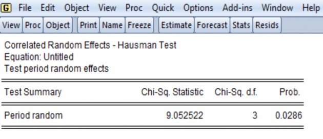
According to the results of Table 3.5, we see that Cross-section random has the corresponding p_value probability 0.0286 < 0.05, so we reject the hypothesis Ho, that is, Xitv is not correlated with eit. That is, the FEM model is more suitable.
4.4.5 Verification of Variation
To test whether the variance of the model changes or not, the author uses the condition of the stationary series, first recalling the stationary series:
A time series is said to be stationary if the expectation and the variance are constant over time, and the covariance between the two observation periods (in the series under consideration) depends only on their lag distances and not on depends on the time of calculation.
Mathematically, a series Yt is said to be stationary if all three conditions are satisfied:
(𝑌𝑡) = (∀𝑡)
(𝑌𝑡) = (𝑌𝑡 − )2 = 2 (∀𝑡)
𝐶𝑜𝑣(𝑌𝑡,𝑌𝑡−𝑘) = [(𝑌𝑡 − 𝜇)(𝑌𝑡−𝑘 − 𝜇)] = (∀𝑡)
A non-stationary series is a series that violates at least 1 of the 3 conditions above Test of Variance:
We consider the residual stationarity of the model with the following assumptions
H0: the residuals of the model are not stationary
H1: residual of stop pattern
Table 4.7: Variance test
According to the results of the above table: the residual of the model has probability P-value < 0.05, so we reject the null hypothesis H0, or the residual of the stationary model. One of the conditions of the stationary series is that the variance does not change, so the variance of the model does not change.
4.4.6 Results of regression model according to FEM
As described above, the data used in this study is asymmetric panel data of 28 banks with a period of 11 years. After running the selection test between Pooled, Fem, and Rem models, the final result is the selection of the Fem model. The following is a table of regression results of Fem model with 3 dependent variables HHI, EQ, ASSEST01.
Table 4.8: Results of regression model according to FEM
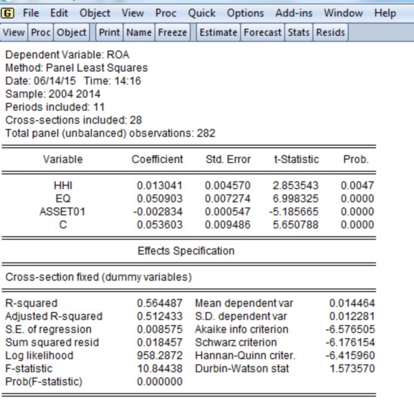
Looking at the model, we see that the auxiliary variables HHI, EQ, ASSET01 all have P-value <0.05. This shows that these variables have a statistically significant impact on bank performance.
4.5 Interpretation of research results
The topic has found a suitable research model to explain the relationship between the variables, and at the same time has tested the appropriateness of the model.
4.5.1 Variable Equity to Total Assets (EQ)
The ratio of equity to total assets (EQ) is positively correlated with bank performance ROA at 1% significance level. This variable reflects the capital structure of each bank. The bank's equity is a buffer against bankruptcy risk, protects the interests of depositors and contributes to the brand and trust of customers. A high equity/total assets ratio means a low debt/total asset ratio, and the bank will significantly reduce the cost of capital such as interest expenses and costs related to capital mobilization.
Reducing costs will directly increase profits. This is also consistent with hypothesis H1.
4.5.2 Bank size variable (ASSET01)
According to research hypothesis H2, bank size has a positive effect on bank performance. Indeed, bank size is used to reflect economies of scale in the market. That is, the larger the bank, the higher the revenue and profit. The results show that the size variable (ASSET01) has a statistically significant negative impact on ROA.
This result is also not surprising because in some situations, too large a bank will reduce profits because it is beyond the control of the bank. Berger et al. (1987) argue that large banks will face a size disadvantage, because as the size increases, the costs also increase. At the same time, Anna and Hoi (2007) with the study of banks in Macao from 1993 to 2007 also show that banks with small scale will have higher ROA.
On the other hand, in Vietnam, banks with large total assets (large scale) often lend to large corporations, use a lot of capital and have many advantages in borrowing relationships, which are mainly state-owned corporations. , these corporations have low business efficiency and banks have to bear the risk when these businesses face financial difficulties. And when lending to large-scale state-owned enterprises, banks usually have to simplify appraisal procedures, and this poses a potential risk of bad debt if the loan enterprises deliberately hide any illegal information. its own benefit. In which, the most popular is the economic case of Vinashin Group. This is the largest economic case in Vietnam today with thousands of billions of dong loss, leaving heavy socio-economic consequences and causing extremely serious impacts on the operations of many important banks. credit system with this group.It can be said that large banks have large provisioning rates for credit risks during the crisis period, which directly reduces profits.
4.5.3 The concentration variable of the loan portfolio
The relationship between ROA and HHI is positive, meaning that the higher the concentration of the loan portfolio, the higher the ROA. In Vietnam, most banks focus on lending in some areas of high profit. For example, the period 2006-2007 was the flourishing period of non-manufacturing industries such as real estate business, securities business, so the credit growth rate in these industries increased sharply in 2007, and the growth rate of profit after tax also peaked. However, entering 2008, due to the influence of the world economic crisis, Vietnam's economy grew slowly, inflation increased again, making lending and deposit activities of banks reduced. decrease, at the same time the bank's risk increases. In addition, looking at Table 2.1, it is clear that commercial joint stock banks with large scale of loan portfolio also mainly focus on the fields of commerce, manufacturing, processing, and personal services.