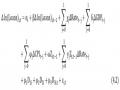
The Asymmetric Effect Of Monetary Policy On The Supply Of Bank Credit

(2009), after taking into account short-term changes, our estimated model is detailed by the following equation:

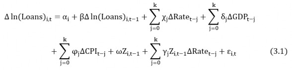
where i = 1,…,N, N is the number of banks, t = 1,…,T, T is the study time, and j = 0,…,k, represents the number of lags. Loans i,t is the credit of bank i in year t.

∆Rate t - j is the first difference of the nominal short-term interest rate, used as an indicator of the monetary policy situation . ∆GDP t – j and ∆CPI t – j are GDP growth rate and inflation rate respectively, representing the demand for credit. The bank features are measured by the vector Z i,t - 1 . Finally, we take into account fixed effects across banks, as measured by the intercept α i .

When studying the bank lending channel in the countries of Central and Eastern Europe, Matousek and Sarantis (2009) introduced a dummy variable in the form of ownership (Own) to determine the different effects. of foreign and domestic banks on overall bank credit growth. However, the operation of foreign banks in Vietnam is still limited, and data on foreign banks is not publicly available. Therefore, we will not include this dummy variable in the model when studying the bank lending channel in Vietnam.

Many researchers have suggested several banking characteristics to determine how sensitive different banks are to changes in monetary policy. According to Matousek and Sarantis (2009), we use three bank characteristics, namely size (Size), liquidity (Liq), and capitalization (Cap) to test the existence of the distributional effects of government. monetary policy among banks in Vietnam, the measurement of these variables is done similarly to Ehrmann et al. (2003) and Gambacorta (2005):

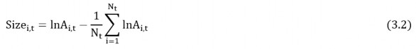
in there:

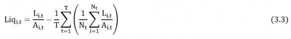
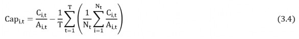
Size i,t represents the size of bank i in period t; Liq i,t represents the liquidity of bank i in period t; Cap i,t represents the capitalization of bank i in period t;

N t is the number of banks in period t.

A i,t is the total assets of bank i in period t;

Li ,t is the total liquid assets of bank i in period t. C i,t is the total equity of bank i in period t.

Bank size is defined as the natural logarithm of total assets, liquidity is measured as the ratio of liquid assets to total assets, bank capitalization is measured as the ratio of total capital owners on total assets. All three bank characteristics are normalized with respect to their mean across all banks in the sample. The construction of the calculation formula for the banking characteristics in equations (3.3) and (3.4) sets the common average of liquidity and capitalization to zero across time and across banks. This way, time changes in liquidity and average capitalization are not eliminated in the analysis. On the other hand, the interpretation of the size feature in equation (3.2) does not include the rapid growth of the banking sector, by setting the average size of a bank to zero for each period. To avoid having many different values of the bank characteristic variables for a

For a given period, only a lag of bank-specific variables is included in the regression model.

The most important feature of the model is the inclusion of interaction terms, which are the product of the monetary policy index and the bank-specific features. As has been discussed, the interaction measure of bank characteristics with short-term interest rates captures the distributive effects of the monetary policy situation. It is assumed that banks with small size, illiquidity, and low capitalization will be more responsive to changes in monetary policy than banks with large size, good liquidity, and capital. high chemistry. Therefore, we test the relevant hypotheses about the existence of a bank lending channel by providing evidence:

- First, ∂ 2 Loans i,t / ∂∆Rate t – j ∂Size i,t – 1 > 0. This implies that the lending activities of large banks are less sensitive to changes changes in monetary policy relative to the lending practices of small banks. Kashyap and Stein (1995, 2000) and Kishan and Opiela (2000) argue that small banks are more susceptible to information asymmetry problems than large banks. This will make small banks more sensitive to monetary policy shocks, since unlike large banks can easily increase non-deposit capital in response to money shocks. bad.

- Second, ∂ 2 Loans i,t / ∂∆Rate t – j ∂Liq i,t – 1 > 0. This implies that banks with high liquidity are less sensitive to changes in monetary policy relative to banks with low liquidity. Kashyap and Stein (2000) and Ehrmann et al. (2003) suggest that in the face of a tightening monetary shock, highly liquid banks can protect their credit portfolio by reducing liquid assets, in when banks are illiquid can't do the same.

- Finally, ∂ 2 Loans i,t / ∂∆Rate t – j ∂Cap i,t – 1 > 0. This implies that high-cap banks are less sensitive to changes in policy monetary policy compared to low-cap banks. Peek and Rosengren (1995) and Kishan

and Opiela (2000, 2006) argue that banks with weak capital will reduce their credit supply more than well-capitalized banks after a monetary tightening, due to limited ability to their access to non-deposit capital.

Regarding macroeconomic variables, similar to Matousek and Sarantis (2009), we use short-term operating interest rates to represent the monetary policy index, and price changes (changes in CPI) and real GDP growth to account for the impact of the macroeconomic environment on credit demand.

Table 3.1. Variables in the model and expected correlation

Variable	Expected about the sign	Explain
ln(loans) i,t – 1	+	Credit growth last year created inertia credit growth next year (Altunbas et al., 2009)
∆GDP t – j	+	Economic growth will increase the demand for credit, leading to an increase in the supply of credit (Kashyap et al., 1993)
∆CPI t – j	+	Rising prices will increase the demand for credit, leading to an increase in the supply of credit (Benkovskis, 2008).
∆Rate t-j	-	Rising interest rates will limit credit growth (Bernanke and Gertler, 1995)
Size i, t – 1	+/-	The larger the commercial bank, the higher or lower the credit growth (Kashyap and Stein, 1995)
Liq i,t – 1	+	The bigger the bank liquidity last year, the better credit extension next year (Stein, 1998)

Maybe you are interested!

Cap i,t – 1	+	The larger the bank capitalization last year, the more open it will be credit extension next year (Van den Heuvel, 2002)
Size i, t – 1 Rate t – j	+	The smaller the banks, the more sensitive they are to changes in monetary policy (Kashyap and Stein, 2000)
Liq i,t – 1 Rate t – j	+	The more illiquid banks are, the more sensitive they are to changes in monetary policy (Ehrmann et al., 2003)
Cap i,t – 1 Rate t – j	+	The lower the capitalization of banks, the more sensitive they are to changes in monetary policy (Kishan and Opiela, 2006)

Source: Compiled from previous studies

3.2. Research Methods

The model (3.1) used in the study is a dynamic panel model (Dynamic Panel Model). Due to the dynamics of the model, if the model is estimated by OLS, FEM or REM methods, whether we admit or not admit the correlation between the separate effects α i (of each bank, constant over time). time) and the independent variable, the estimation results are still biased and unstable because in model (3.1) there is also a correlation between the error ε i, t and the lagged variable of the dependent variable Δln(loans). i,t - 1 (used as independent variable) was not processed, causing additional endogeneity problems for the model (Nickell, 1981).

In order to overcome these shortcomings, Arellano and Bond (1991) proposed a solution using the Difference Generalized Method of Moments (DGMM) model, that is, estimating the model (3.1) in the form of first difference and using the lags of the dependent variable and of the independent variables endogenously as instrumental variables. By converting the regressors to first difference , the separate effect α i was eliminated, and the use of lags of the dependent variable was eliminated.

dependencies and of the independent variables are endogenous as instrumental variables allowing to create orthogonal conditions between the error εi ,t and the explanatory variables (including the lagged variable of the dependent variable) Δln(loans) i,t - 1 ), ie remove the correlation between them to solve the potential endogeneity problem.

However, Blundell and Bond (1998) suggest that when the dependent variable has a high correlation between the present value and the value in the previous period, and the number of periods is not too long, then the GMM (1991) model is not efficient, the instrument variables used are evaluated as not strong enough. Blundell and Bond (1998) extended the GMM (1991) model by considering the system of two models simultaneously – the basic model (Level Equation) and the first-differentiation model (First – Difference Equation) – collectively called System Generalized Method of Moments (SGMM) model. For the basic model, we will use the instrumental variable that is the lagged variables of the first difference of the explanatory variables, for the differential model, we will use the instrumental variable that is the lagged variables of the explanatory variables ( The explanatory variable includes the lagged variable of the dependent variable Δln(loans) i,t – 1).

In addition to the endogeneity problem caused by the lagged dependent variable on the right hand side of equation (3.1), another endogeneity problem arises, since bank credit can be strongly correlated with other items on the balance sheet and are therefore also strongly correlated with bank-specific characteristics (Benkovskis, 2008). Meanwhile, we assume that the monetary policy index, output growth, and price growth are independent of individual bank credit growth. In fact, credit growth of the largest banks may still have some influence on domestic macroeconomic variables. However, assuming domestic macroeconomic variables as strictly exogenous does not significantly change the research results (Benkovskis, 2008).

To explain the autoregressive nature and overcome the endogeneity of the model (3.1), including the endogeneity of the lagged dependent variable and the possible endogeneity of the bank-specific feature variables , the systematic GMM method (SGMM, 1998) is used in our study. Besides handling well the endogeneity problem by instrumental variables, the SGMM method is also suitable for the data.

table with a short time series T and a large number of N firms. In this study, we use panel data with a short period of only 10 years but a relatively large number of banks. Therefore, the use of the SGMM method is also consistent with our study in terms of data.

Another important issue is choosing between 1-step and 2-step SGMM estimates. The difference between these two estimates lies in the characteristics of an individual weight matrix; 2-step estimation using the remainder of 1-step estimation should be more efficient. However, Benkovskis (2008) recommends that the standard error of the 2-step estimate tends to be biased down in small samples, so the results of the 1-step estimate will be used in our paper. I.

The estimates in the study were performed using Stata 12 software, using the xtabond2 command introduced by Roodman (2009) with robust option. The robust option is used when the residuals of the model have variable variance. Usually the residuals in GMM will have the problem of HAC (variable residual variance and autocorrelation) so using robust is appropriate. The robust option will estimate with the actual value of the covariance matrix of the parameters. The actual errors of the estimated coefficient will be calculated, thereby increasing the reliability of the estimated coefficient.

The SGMM (1998) model is only considered suitable when two conditions are satisfied. First, there are restrictions on overidentifying restrictions, that is, to determine the appropriateness of the instrumental variables, to test the non-existence of the correlation between the instrumental variables and the error. . Second, there is no quadratic autocorrelation in the first difference residuals.

To test the appropriateness of the SGMM, the Hansen test (1982) on the over-determined limit and the Arellano-Bond test (1991) on the autocorrelation phenomenon were used. First, the Hansen (1982) test on the over-determined limit in the SGMM estimate is a chi-square test of the validity of the instrumental variable. Good instrumental variables must be consistent and valid, i.e. correlated with endogenous regressors while at the same time orthogonal to residuals (Baum et al., 2003). Hypothesis H 0 of Hansen test is: valid instrumental variable . Therefore, the p-value of the Hansen statistic

the bigger the better. Next, the Arellano - Bond test (1991) on autocorrelation in residuals AR(1) and AR(2), has the hypothesis H 0 is: no autocorrelation and is applied to differential residuals. . The AR(1) process test in first difference usuallyrejects the null hypothesis H0 . This is because ∆ε i,t = ε i,t – ε i,t – 1 and ∆ε i,t – 1 = ε i,t – 1 – ε i,t – 2 , both have ε i ,t - 1 . So the AR(2) test is more important because it tests autocorrelation at all levels. In this study, since the estimation method involves taking the first difference, there should be first order autocorrelation, but no second order correlation in the remainder of the order difference equation. best. Therefore, the higher the p-value of the Arellano–Bond test for AR(2), the better.

3.3. Research data

The study conducted regression estimation of panel data. Data sources are collected from audited annual consolidated financial statements of 30 Vietnamese commercial banks for the period from 2005 to 2014 2 . In which, there is 1 state-owned commercial bank, 4 banks with a large state ownership rate, and 25 joint stock commercial banks. The research sample does not include the Vietnam Development Bank and the Bank for Social Policies, which are specialized banks in providing credit to the government's priority subjects, so the credit activities of banks are not included. This is less affected by monetary policy decisions. Joint Venture Banks, Foreign Banks and Foreign Bank Branches in Vietnam are also not included in the analysis because the activities of this group of banks are still limited.3 , moreover, the data of this group of banks is not publicly available.

Regarding the selection of figures from the consolidated financial statements instead of those from the separate financial statements, we believe that the consolidated financial statements are the basis for our consideration.

2 See Appendix C.1 for a list of banks in the sample.

3 Total assets of Joint Venture Banks and Foreign Banks in Vietnam account for only about 11% of the total assets of the whole industry according to statistics of the State Bank as of July 31, 2013.

operations of modern banks. The main reason is that nowadays most banks are developing in the direction of multi-industry and multi-field corporations, so the separate financial statements cannot reflect the financial position as well as the real business situation of the bank. for these banks, only the consolidated financial statements can meet the above objectives.

Due to limitations in terms of data disclosure and collection, as well as the period from 2005 to 2014 was a period of witnessing the ups and downs of Vietnam's banking industry, with the first phase of the research The study marked a strong development when there were a series of new banks entering the industry, while the later period of the research period showed a leveling off with signs of recession when a series of banks had to face new requirements. demand for reforms, mergers, or exits from the industry. Therefore, there are some banks that do not have complete data during the survey period, so the research data collected is unbalanced panel data with 30 banks and 295 observations.

The balance sheet data of each bank is collected from the websites of securities companies as well as the banks themselves. The indicators used to measure the bank credit growth variable and the bank-specific variables that we use in the research model are secondary data, calculated from the items on the table. balance of each individual bank 4. In which, bank credit is defined as total loans to customers and includes problem loans. The size of a bank is measured by the total assets on its balance sheet. Liquid assets include cash and cash equivalents, deposits with the State Bank, deposits with and loans to other credit institutions, trading securities, investment securities, and financial instruments. derivatives and other financial assets. Capital is defined as the sum of capital and funds (similar to Matousek and Sarantis, 2009).

As mentioned in Section 3.1, the monetary policy index in our research model is represented by changes in short-term operating interest rates.

4 See Appendix C.2 for bank balance sheet data.

In terms of policy interest rates, there are three main interest rates in Vietnam: average interbank rate (VNIBOR), refinancing rate, and rediscount rate. However, the discount door and refinancing loans in Vietnam are not very active and effective, while the interbank market is the main operating channel of the State Bank in implementing monetary policy. . Therefore, the average interbank interest rate is often used as a proxy for the interest rate of monetary policy in Vietnam (Tram Thi Xuan Huong et al., 2014). Central banks around the world also use the average interbank interest rate as a proxy for monetary policy (Disyatat and Vongsinsirikul, 2003; Benkovskis, 2008). In this study,

The sample period spans from 2005 to 2014. This seems to be a sufficiently long period because it covers the entire cycle of monetary policy, i.e., periods of monetary tightening and easing currency (see Figure 3.1).

Average interbank interest rate for 3-month term (%)

ten

-2

-4

-6

-8

-ten

twelfth

ten

2005 2006 2007 2008 2009 2010 2011 2012 2013 2014

DRATE (differentiation, left column)

RATE(value, right column)

Figure 3.1. Monetary policy index of Vietnam for the period 2005 - 2014

Source: Ho Chi Minh City University of Economics Data Center

There are two reasons for us to choose 2005 as our research landmark. Firstly, 2005 was the year when a number of important legal documents were born, serving as a premise for the management, administration and operations, which greatly influenced the business activities of enterprises as well as organizations. institutions operating in the credit sector such as Enterprise Law, Competition Law, etc. Second, because of the availability of data and the requirements of the variables in the research model.

Data on average interbank interest rates and annual macroeconomic situation (real output growth GDP and CPI inflation) for the period from 2005 to 2014 are collected from the University Data Center Economy of Ho Chi Minh City 5 . The data is collected and sorted by panel data.

The table data structure is composed of two components: a cross data component and a temporal data component. Tabular data is now widely exploited and used, because it overcomes the lack of data, overcomes the disadvantages of temporal data, cross-sectional data, and importantly, the tabular data feature exhibits diversity. format and richness, helping the estimation results have high reliability.

Table 3.2. Descriptive statistics of variables

Variable	2005 - 2014 (N = 295)
Variable	The average value	Smallest value	The greatest value	Standard deviation
Loan (Lan Loan)	16.6728	11.0602	20.1011	1.6151
Size (ln assets)	17.3272	11.8835	20.3623	1.6212
Liquidity (equity/asset)	0.3751	0.0400	0.7493	0.1404
Capitalization (capital/asset)	0.1231	0.0291	0.7121	0.0926
Short-term interest rate (rate)	9.0271	3.7400	16.2300	3.4562
GDP growth	6.1977	5.2474	7.5473	0.7624
CPI . inflation	10.2209	4.0898	23.1221	5.6673

Source: Author's calculations

5 See Appendix C.3 for macroeconomic data.

The results of descriptive statistics of the study data are presented in Table 3.2. In general, the development of the banking industry is still uneven, the disparity in asset size, total credit, ratio of liquid assets to total assets, and the ratio of equity to total assets still quite large.

Specifically, the average credit growth of commercial banks (calculated by the natural logarithm of total credit) is 16.67%, varying strongly from 11.06% to 20.10%, this figure is equivalent to financial growth. Banks' assets (measured by the natural logarithm of total assets) is 17.33%, ranging from 11.88% to 20.36%, which shows that the growth in size of the banking industry is accompanied by growth. credit to the economy. Meanwhile, the liquidity ratio and the bank capitalization ratio (measured by the ratio of liquid assets to total assets and the ratio of equity to total assets) are generally less volatile, with deviation relatively low standards (0.14 and 0.09). The average short-term interest rate is 9.03% and ranges from 3.74% to 16.23%, shows that the period 2005 - 2014 was a period when Vietnam's monetary policy had many great fluctuations along with the State Bank's efforts in stabilizing the money market. However, it seems that the performance of the economy is still not efficient, although the credit growth rate is relatively high (average 16.67%) but the real GDP growth rate is only 6.20%, meanwhile The average CPI inflation rate is quite high at 10.22%, and fluctuates quite strongly from 4.09% to 23.12% (with a standard deviation of 5.67). This shows that the influence of bank credit on inflation is larger than that of economic growth, implying that the economy's ability to absorb bank credit sources is still not good. Although credit growth is relatively high (16.67% on average), the real GDP growth rate is only 6.20%, while the average CPI inflation rate is quite high at 10.22%, and fluctuates relatively. strong from 4.09% to 23.12% (with a standard deviation of 5.67). This shows that the influence of bank credit on inflation is larger than that of economic growth, implying that the economy's ability to absorb bank credit sources is still not good. Although credit growth is relatively high (16.67% on average), the real GDP growth rate is only 6.20%, while the average CPI inflation rate is quite high at 10.22%, and fluctuates relatively. strong from 4.09% to 23.12% (with a standard deviation of 5.67). This shows that the influence of bank credit on inflation is larger than that of economic growth, implying that the economy's ability to absorb bank credit sources is still not good.

CHAPTER 4

RESEARCH RESULTS

4.1. The asymmetric effect of monetary policy on the supply of bank credit

To learn about the role of the bank lending channel in the transmission of monetary policy of the State Bank of Vietnam, we need to understand how monetary policy affects the supply of bank credit. According to the theory of lending channels, the impact of monetary policy on the supply of bank credit has an important distributional nature, different banks in terms of size, liquidity, capitalization will react differently to a given loan. tightening monetary shock. To find empirical evidence on the asymmetric effect of monetary policy on the supply of bank credit, we estimate the model (3.1) using the SGMM method as mentioned in Chapter 3. Ehrmann and Worms (2004) argue that monetary policy has lag in the impact on other variables in the economy, similar to Matousek and Sarantis (2009), in this study, we also tested with various lags for the explanatory and dependent variables, but the tests show that longer lags are not statistically significant, so one lag is enough for Vietnam. The model (3.1) with a delay is specified as follows:

The model's estimates are presented in Table 4.1, which shows the regression coefficients and the significance level of the variables 6 . For bank characteristics, we estimate the model with each individual feature (column 1 – column 3), then with each feature pair (column 4 – column 6), and finally with all three features. characteristics together (column 7). In

6 Detailed results of the estimates are presented in Annex B.1 – Annex B.7.

For each regression we use all endogenous independent variables at time t - 2 as instrumental variables 7 .

We will analyze the results presented in Table 4.1 in turn according to the following contents:

- The first is the results of Hansen's test and Arellano Bond's test for the concordance of the SGMM estimates.

- Next, we will consider the fixed effects across banks, bank credit growth, the direct impact of monetary policy on bank credit growth, the impact of credit demand on bank credit growth, the impact of bank characteristics on bank credit growth, as well as the distributional effects of monetary policy on bank credit growth.

- Finally, we will conduct a selection bias test to ensure the reliability of the analyzed results.

According to Matousek and Sarantis (2009), normally for annual data, when an endogenous independent variable in the regression model is at time X t - i , the instrumental variable will be X t - i - 1 .

	Size (1)	Liq (2)	Cap (3)	Size Liq (4)	Size Cap (5)	Liq Cap (6)	Size Liq Cap (7)
Loans(1)	0.5500***	0.8900***	0.8810***	0.5570***	0.5750***	0.9200***	0.5570***
Rate	-0.1210***	-0.0071	-0.0156	-0.1250***	-0.1170***	0.0010	-0.1290***
Rate(1)	0.0383	-0.1140***	-0.1150***	0.0356	0.0517	-0.1220***	0.0650
GDP	0.2360**	0.5940***	0.6140***	0.2560**	0.2110	0.6150***	0.1900
GDP(1)	-0.3680***	-0.2130***	-0.2360***	-0.3770***	-0.3390***	-0.1950***	-0.3490***
CPI	0.0804***	0.0227*	0.0307**	0.0854***	0.0759***	0.0182	0.0822***
CPI(1)	0.0032	0.1020***	0.1050***	0.0071	-0.0064	0.1070***	-0.0134
Size(1)	0.3160***			0.3190***	0.3060**		0.3200**
Size(1)*Rate	0.0063**			0.0059**	0.0135**		0.0139**
Size(1)*Rate(1)	0.0016			0.0014	-0.0009		-0.0008
Liq(1)		0.3690		-0.1590		0.9290	-0.0458
Liq(1)*Rate		-0.0015		-0.0130		-0.0119	0.0155
Liq(1)*Rate(1)		-0.0015		-0.0087		-0.0431	-0.0399

Table 4.1. Estimations of equation (4.1) using bank data

Date published: 10/04/2022