Viterbi Type Algorithm To Find The Best Analysis

The thesis has not been tested on complex sentences, which are sentences with two or more subject clusters but one cluster covers the remaining clusters, for example “the shirt you bought yesterday was very nice” with two subject clusters “you bought” “beautiful shirt”, the phrase “beautiful shirt” covers the rest. In fact, some cases can already be analyzed with our compound sentence analyzer, like the sentence “It says it doesn’t go anymore”. However, some cases need to use machine learning method to recognize gender. clause term.

3.2.5. Computational complexity

According to Sleator [111], the time cost of the association analysis algorithm (when not pruned) is for a given grammar of O(n3) where n is the sentence length (the number of words in the sentence), the cost This is also equivalent to the time cost of parsing algorithms using context-free grammars. When parsing natural language, n is not large, so most of the time cost is due to finding matching rules in the grammar. If the grammar size is also considered, the association analysis algorithm has a cost of O(n3m), m is the average number of selected forms of the words in the sentence. Meanwhile, the complexity of CYK and Earley algorithms for context-free grammar according to Jurafsky [70] is O(n3 |G|), |G| is the production number of the context-free grammar.

The main time cost is due to the combing stage. In Vietnamese, because words do not change morphology, each word must have many relationships with words indicating tense, form, number…, The average number of selected forms (not trimmed) of each word is about 10,000. From [111] it can be seen that the pruning algorithm has a cost of O(nm).

If the discourse segmentation process divides the sentence into k clauses, the average length of each clause is n/k, the average time cost will be reduced k2 times. The cost of discourse segmentation is O(n), the cost of traversing the discourse tree is a binary tree consisting of k/2 leaf nodes (no leaf node traversal) corresponding to k propositions not exceeding O(k). larger, the time cost will be smaller. However, if k equals 1, the cost will be greater than the cost of parsing a single sentence.

Experiments with the first set of sample sentences in Table 3.5, show that the time to analyze the sample set by linking word association is 296,153 milliseconds, while the time to analyze that sentence by analyzing each clause separately is 217,324 milliseconds, which is significantly less than word association analysis.

3.3.Remove ambiguity

As discussed in chapter 2, Jurafsky [70] addresses two major problems in syntactic ambiguity: component ambiguity and conjugate ambiguity. Component ambiguity occurs when a structure can join different parts of the analysis tree, producing different analyses. Cordination ambiguation occurs when phrases are linked together by the conjugation “and”, “or”, “or”…Local ambiguity is also taken into account. when a word can receive labels from different categories. The local ambiguity of the partial association model was resolved during parsing. Unlike other models, the word is not labeled before parsing but is labeled based on the association it joins. A word with multiple meanings will appear in different formulas, but only combinations of words and labels that satisfy the association requirements will be accepted. Thus, the number of associative analyzes of each sentence is significantly smaller than the number of syntactic trees of the context-free model.

Maybe you are interested!

In this section, we deal with the problem of component ambiguity and conjugate ambiguity. For component ambiguity, the thesis has chosen the approach of Lafferty and colleagues [79] with a general description of a trigram probability model. From this description, the thesis must build a de-ambiguity algorithm for its application.

3.3.1. Eliminate component ambiguity

The composition ambiguity problem occurs when a sentence has more than one association analysis. The sentence considered here is a simple sentence. If it is a compound sentence, it will only solve the problem of ambiguity after splitting it into clauses.

According to the trigram model [79], the de-ambiguity reduction is not about calculating the probability of each analysis, finding the sentence with the highest probability, but using the hidden Markov model (HMM) to predict the sentence with the highest probability. Best. The two main problems to be solved for this purpose are:

Find the sentence with the highest probability according to the Viterbi-style algorithm.
Update the probability of the production.

3.3.1.1. Viterbi type algorithm to find the best analysis

In [79], a probabilistic model for association grammar was introduced similar to the one described in Section 1.1.2. for context-free grammar. If in a context-free grammar the basic operation is a rewrite, in a linking grammar the basic operation is to find a link. The production equivalent of a context-free grammar in a linking grammar is a link. Each link depends on two connections: a right connection and a left connection of the same name connecting two words L and R . So the parameter of the linking grammar is:

Pr ( W, d, O | L, R, l, r ) (3.1)

O can take the values →, ←, ↔ representing the direction of the link. It can be understood that: given the word L has a right connection of l and the word R has a left connection r, the parameter is the probability of the event: exists word W between L and R, the selected form d of W is linked. with L or R or both. Probability (3.1) decays to:

Pr ( W, d, O | L, R, l, r ) =

Pr(W | L, R, l, r ) × Pr ( d | W, L, R, l, r ) × Pr ( O | d, t, p, q, l, r ) (3.2)

Since we are dealing with conditional probabilities on a set of events that are too large for a grammar with a natural language vocabulary, it is practically impossible to estimate this probability. Therefore it needs to be approximated by the formula [79]:

Pr ( W, d, O | L, R, l, r ) ≈ Pr (W | L, R, l, r ) × Pr (d | W, l, r ) × Pr (O | d, l, r ) (3.3)

The probability of a link analysis is the product of the probabilities of every link in it. It is now necessary to represent the association analysis L by a set of associations L = {(W, d, O, L, R, l, r)} together with the first membership form d0. The probability of L is:

Pr ( S, L ) = Pr ( W0, d0 ) ∏ Pr ( W, d, O | L, R, l, r )

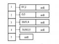
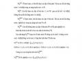
Example: A probabilistic association grammar stores the following parameters (The nth word is the “dummy” word Wn used in the algorithmic analysis in Figure 3.4):

Pr ( I, ( ) ( SV ) ) = 0.7

Pr( buy, (SV)(O), ← | i, Wn , SV, NIL) = 0.06

Pr ( flower, ( O, NcNt3 )( ), ← | buy, Wn , O, NIL) = 0.03

Pr( cotton, (McN)(NcNt3), → | buy, flower, NIL, NcNt3) = 0.05

Pr ( one, ( )(McN), → | buy, cotton, NIL, McN) = 0.06

Pr( cotton, (O, McN)(NcNt3), ↔ | buy, Wn , O, NIL) = 0.00001

Pr ( flower, (NcNt3)( ) ← | cotton, Wn, NcNt3, NIL) = 0.07 (3.4)

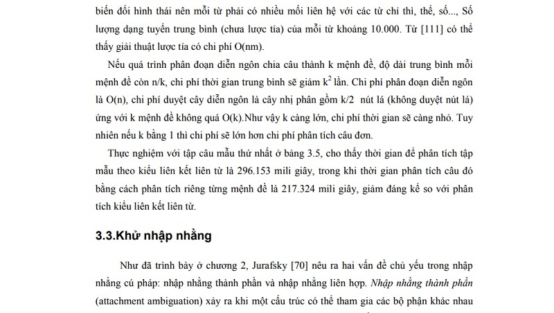
Suppose the sentence “I bought a flower” has two analyzes L1 and L2 as shown in Figure 3.20 below:

Figure 3.20. Two analyzes of the sentence “I bought a flower”

The probability for the L1 analysis (Figure 3.20(A)) is:

Pr (L1) = Pr ( 0, ( )( SV ) ) × Pr ( 1, (SV)(O), ← | 0, 5 , SV, NIL ) ×
Pr ( 4, ( O, NcNt3 )( ), ← | 1, n, O, NIL ) ×
Pr ( 3, (McN)(NcNt3), → | 1, 4, NIL, NcNt3 ) ×
Pr ( 2, ( )(McN), → | 1, 3, NIL, McN )
= 0.7 * 0.06 * 0.03 * 0.05 * 0.06
= 3.78E-5

While the probability of L2 analysis (Figure 3.20. (B)) is:

Pr (L2) = Pr ( 0, ( )( SV ) ) × Pr ( 1, (SV)(O), ← | 0, 5 , SV, NIL ) ×
Pr ( bông, (O, McN)(NcNt3), ↔ | mua, Wn , O, NIL ) ×
Pr ( một, ( )(McN), → | mua, bông, NIL, McN ) ×
Pr ( hoa, (NcNt3)( ) ← | bông, Wn, NcNt3, NIL )
= 0.7 × 0.06 × 0.00001 × 0.06 × 0,7
= 2E-8

If one of the two analyzes had to be selected, L1 would be chosen.

In [79] only probabilistic models are given for grammars associated with inner and outer probabilities similar to forward and backward probabilities in the HMM model. The thesis has proposed a Viterbi-type algorithm for the associative grammar model.

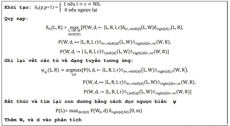
Figure 3.21. Viterbi-style algorithm to predict the analysis with the highest probability

Date published: 01/11/2021