Analysis Of Multi-Group Model According To Customer Characteristics

Table 4.11 Results of EFA analysis of all variables

% of variance

TVE

Cumulative TVE %

KMO=.934		Bartlett test: Sig.=000
Factor	Eigenvalue
first	11,642	40.415	40.415
2	2.873	9,070	49.485
3	1,773	5.097	54.582
4	1.537	4.158	58,740
5	1.424	3,907	62,647
6	1.157	3.111	65,758
…	.....	.....	.....

Maybe you are interested!

• The Need To Study The Loyalty Of Depositors At Vietnamese  Commercial Banks
• Actual Situation Of Deposit Mobilization Activities Of Vietnamese Commercial Banks In The City. Ho Chi Minh
• The influence of corporate social responsibility on the loyalty of customers depositing money at Vietnamese commercial banks - 5
• Suggestions On Implementing Social Responsibility Customer-Oriented Approach
• The influence of corporate social responsibility on the loyalty of customers depositing money at Vietnamese commercial banks - 8
• The influence of corporate social responsibility on the loyalty of customers depositing money at Vietnamese commercial banks - 9

( Source: author's calculation from SPSS, appendix 7)

First, KMO=.934  >  .5 so EFA analysis is appropriate for real data. Bartlett test has statistical significance (Sig=.000 < .005) so the variables are correlated with each other in the population.

Second, the EFA results analyzed 6 factors and the Eigenvalues ​​are all greater than 1 (the smallest coefficient is 1.157), thus retaining all 6 factors as the original analysis, no need to reduce the set of factors. . The total variance extracted is 65.758% (greater than 50%), that is, 65.758% of the variation of the factors is explained by the observed variable.

Table 4.12 Matrix of components

Factor Observed variables	Definitive identification	Faithful	Corporate Social Responsibility	Feelings of FIRE	Satisfaction FIRE	Loyalty FIRE
ND3 ND5 ND4 ND6 ND2 ND1	.907 .865 .859 .780 .721 .637
NT5 NT3 NT4		.852 .845 .826

NT2 NT1		.742 .718
TN3 TN4 TN2 TN5 TN1			.905 .860 .822 .779 .770
CX4 CX3 CX2 CX1				.874 .816 .812 .714
HL3 HL2 HL4 HL1					.793 .789 .642 .620
TT3 TT4 TT1 TT2						1.025 .742 .605 .587

( Source: author's calculation from SPSS, appendix 7)

Third, the factor loading coefficients of the 6 download factors are all greater than 0.5 (the lowest is 0.587), showing that the study has achieved practical significance.

Fourth, the difference between the loading coefficients among the factors is at least 0.3 ( see Appendix 7),  satisfying the condition for each observed variable to exist in the centralized model explaining for a single factor.

With the above indicators, it can be concluded that the factor analysis model has complete practical significance, high explanatory capacity for reality, and forms 6 similar meaningful factors in the proposed research model. . Six factors including 28 observed variables were kept for CFA analysis in the next step.

4.5.4 Confirmatory factor analysis CFA

The author conducts confirmatory factor analysis for 6 concepts in the research, and uses 5 criteria in the process of testing the scale. First: evaluate the relevance of the data to reality. Second: aggregate reliability and total variance extracted. Third: test discriminant validity. Fourth: verify the convergence value of the scale. Finally, check the unidirectionality of the model. The first CFA results are presented as shown in Figure 4.3:

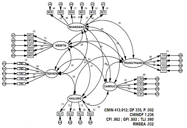
Figure 4.3 Results of 1st Normalized CFA analysis

The analysis results show that, with Chi-square test, the model has no significant difference at the 5% level (P=.002). However, other conformity measures were satisfactory (CMIN/DF= 1.236; GFI=.892; TLI =.980; CFI = .982; RMSEA = 0.032). The CMIN/DF, TLI and CFI indexes are all at very good acceptance levels, while the GFI indexes are only in the temporarily acceptable zone. The normalized weights λ of the measured variables are quite high, with no index lower than 0.5 (the lowest index is .652 of the  ND1 variable)  and reach the level of statistical significance. The RMSEA index = .032 presents very good results, demonstrating high compatibility with market data.

However, the CFA results also show that some errors in the model have a large correlation. When the errors have a large correlation with each other, it is possible to improve the research model. Specifically, some error pairs have high MI (Modification Indices) such as e12 and e13 (MI=10.978), e7 and e8 (MI=7,519), e15 and e16 (MI=6.612), e2 and e5

(MI=5.732), e2 and e3 (MI=4.787). The significance of the MI index is that when these errors are hooked together, the Chi-squared will decrease by exactly the same amount as MI. As a result the model will be improved. The results of the second CFA analysis after hooking the errors in the normalized model are shown in  Figure 4.4.

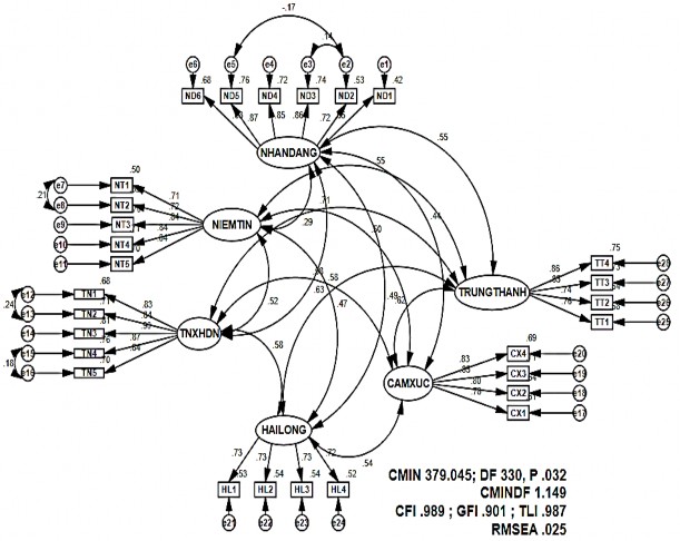
Figure 4.4 The critical model after joining errors has a large correlation coefficient

First,  test the degree of conformity with reality. The model in Figure 4.4 after error matching has a large MI index that has improved compared to the model in Figure 4.3. Although, P has increased significantly (P=.032), the Chi-squared test is still not significant at the 5% level. However, the indices CFI=.989, GFI=.901, TLI=.987 show very good results, all

all indexes are greater than 0.9 as required. The index RMSEA=.025, CMIN/DF=1,149 with a sample size of 236 demonstrates a very high degree of agreement between the data and reality.

Table 4.13 Indicators for testing the reliability of the scale

Concept			i_	i2_	1- i 2 _	Index	Value
Corporate Social Responsibility
TN1	<---	TN	0.83	0.68	0.32	α	0.935
TN2	<---	TN	0.84	0.71	0.29	c_	0.935
TN3	<---	TN	0.90	0.81	0.19	vc_	0.732
TN4	<---	TN	0.87	0.76	0.24
TN5	<---	TN	0.84	0.70	0.30
Customer identification
ND1 ND2	<--- <---	ND	0.65	0.42	0.58	α	0.913
		ND	0.73	0.53	0.47	c_	0.914
ND3	<---	ND	0.86	0.74	0.26	vc_	0.643
ND4	<---	ND	0.85	0.72	0.28
ND5	<---	ND	0.87	0.76	0.24
ND6	<---	ND	0.83	0.68	0.32
Customer confidence
NT1	<---	NT	0.71	0.50	0.50	α	0.895
NT2	<---	NT	0.72	0.52	0.48	c_	0.895
NT3	<---	NT	0.84	0.70	0.30	vc_	0.625
NT4	<---	NT	0.84	0.71	0.29
NT5	<---	NT	0.84	0.70	0.30
Customer's feelings
CX1	<---	CX	0.78	0.61	0.39	α	0.888
CX2	<---	CX	0.80	0.64	0.36	c_	0.889
CX3	<---	CX	0.85	0.71	0.29	vc_	0.666
CX4	<---	CX	0.83	0.69	0.31
Customer satisfaction
HL1	<---	HL	0.73	0.53	0.47	α	0.819
HL2	<---	HL	0.74	0.54	0.46	c_	0.820
HL3	<---	HL	0.73	0.54	0.46	vc_	0.532
HL4	<---	HL	0.72	0.52	0.48
Customer Loyalty
TT1	<---	TT	0.76	0.58	0.42	α	0.877
TT2	<---	TT	0.74	0.54	0.46	c_	0.881
TT3	<---	TT	0.85	0.73	0.27	vc_	0.649
TT4	<---	TT	0.86	0.74	0.26

( Source: author's calculations from SPSS and Excel)

Second,  evaluate the combined reliability ( ρc ) and the total variance extracted ( ρ vc ). The scale is reliable when the combined reliability values  ​​ c  and the total variance extracted   vc  reach >0.5 (Hair et al., 2010) and the combined reliability  ρ c  ≥ Cronbach's alpha ( Hair et al., 2010) a) . Where i  is the normalized weight of the i  -th observed variable; p is the number of observed variables of the scale

( ∑ 2 _  

(∑ )

2)_

measure  : = 

=1

) _

; =  =  1  _

(  _ _ _

2___

2  _

(∑ )

2)+∑_

( 1− 𝑖 2 )

=1

) +

=1 (1− 𝑖  )

=1

=1

Calculation results from table 4.13 show that all concepts have aggregate reliability and total extracted variance is greater than 50% (lowest is 82% and 53.2% respectively), so the indexes satisfy all requirements. required conditions. Besides, the concepts in the model also have composite reliability ≥ Cronbach's Alpha value. Combining the values, the scales in the research model have achieved reliability.

Third,  evaluate the discriminant value. In this study, the scales built do not include many component concepts. Therefore, the author only evaluates the external discriminant value, that is, between external concepts. From the correlation coefficient between variables (r), calculate the standard deviation (SE), CR and Pvalue according to the formulas: SE=SQRT((1-r 2 )/(n-2)) ; CR=(1-r)/SE; P_value

=TDIST(CR, n-2, 2), where n is the sample size.

Table 4.14 Correlation coefficients between concepts

Concept			r	SE	CR	P-value
ND	<-->	NT	0.288	0.063	11.373	0.000
ND	<-->	TN	0.633	0.051	7.252	0.000
ND	<-->	CX	0.436	0.059	9.587	0.000
ND	<-->	HL	0.485	0.057	9,008	0.000
ND	<-->	TT	0.549	0.055	8.254	0.000
NT	<-->	TN	0.518	0.056	8,620	0.000
NT	<-->	CX	0.496	0.057	8.879	0.000
NT	<-->	HL	0.471	0.058	9.173	0.000
NT	<-->	TT	0.549	0.055	8.254	0.000
TN	<-->	CX	0.579	0.053	7.899	0.000
TN	<-->	HL	0.580	0.053	7.887	0.000
TN	<-->	TT	0.711	0.046	6.287	0.000
CX	<-->	HL	0.542	0.055	8.337	0.000
CX	<-->	TT	0.619	0.051	7.421	0.000

HL

<-->

TT

0.576

0.053

7,934

0.000

( Source: author's calculations from Amos and Excel)

The correlation coefficients and standard deviation are both different from 1 and have statistical significance at 1% significance level, so the research concepts achieve discriminant validity.

Fourth,  evaluate the convergence value of the scale . The scale reaches the convergent value when the observed variables of a research concept have high correlation or high standardized λ (≥0.5) and reach statistical significance (P < 0.05). Observing from the critical model in Figure 4.4, we see that the normalization coefficients of the observed variables are all greater than .5 (the lowest coefficient is .65) and these coefficients are statistically significant P= .000 (see  Appendix 9 ) so it can be concluded that the scales used in the model reach the convergent value.

Fifth,  the unidirectionality of the scale set . The scale is unidirectional when there is no correlation between the errors of the observed variables. The critical model ( Figure 4.4 ) shows that the scale of 3 research concepts is unidirectional. Those scales are: customer satisfaction, emotion, loyalty. Particularly, the scale of the concept of CSR, customer identification, and customer trust has a relationship between error pairs (e12 and e13; e7 and e8; e15 and e16; e2 and e5; e2 and e3), so it is not achieve unidirectionality.

4.5.5 Theoretical model testing by SEM . analysis

4.5.5.1 Testing the theoretical model

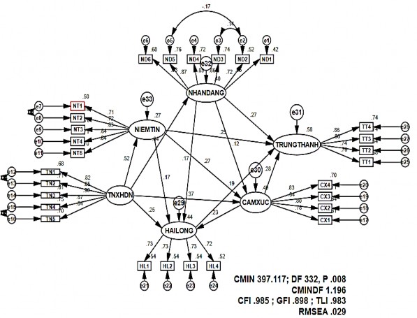
Figure 4.5. SEM results for theoretical model (normalized)

The results of the linear structure analysis show that the research model has a Chi-squared statistical value of 397,117 with 332 degrees of freedom, P = .008. If adjusted for degrees of freedom with CMIN/df = 1.196 < 3, meet the requirements for compatibility. Other indicators such as CFI = .985 > .9, TLI=.983 >.9, RMSEA = .029 < .05 met very well. Although the GFI=.898 value is not greater than .9, the difference is not significant (.002). Therefore, it can be concluded that the model fits the market data.

4.5.5.2 Estimating the theoretical model using Bootstrap

Bootstrap is an iterative alternative sampling method where the initial template acts as the crowd. In order to evaluate the reliability of the estimates, in quantitative research methods by sampling method, we usually have to divide the sample into two subsamples: a part used to estimate model parameters and part for re-evaluation. Or maybe re-evaluate the study

by another sample. However, these methods are time-consuming and costly because the requirements in SEM analysis require large sample sizes (Nguyen Khanh Duy, 2009). In such cases, Bootstrap is the right alternative. This study uses the Bootstrap method with the number of repeated observations N = 500. AMOS software will now select 500 observations according to the substitution method from the crowd of n=236 observations.

Table 4.15 Bootstrap estimation results with N = 500

Relationship			SE	SE-SE	Mean	Bias	SE-Bias	|CR|
NT	<---	TN	0.070	0.002	0.514	-0.008	0.003	2.67
ND	<---	TN	0.047	0.002	0.634	-0.002	0.002	1.00
CX	<---	TN	0.090	0.003	0.365	-0.004	0.004	1.00
CX	<---	ND	0.072	0.002	0.125	0.003	0.003	1.00
CX	<---	NT	0.076	0.002	0.266	-0.001	0.003	0.33
HL	<---	TN	0.103	0.003	0.255	0.000	0.005	0.00
HL	<---	ND	0.082	0.003	0.171	-0.001	0.004	0.25
HL	<---	CX	0.086	0.003	0.231	0.001	0.004	0.25
HL	<---	NT	0.075	0.002	0.168	-0.005	0.003	1.67
TT	<---	NT	0.067	0.002	0.271	0.002	0.003	0.67
TT	<---	CX	0.076	0.002	0.282	-0.002	0.003	0.67
TT	<---	HL	0.091	0.003	0.188	0.003	0.004	0.75
TT	<---	NT	0.072	0.002	0.243	-0.002	0.003	0.67

( Source: author's calculations from Amos and Excel)

Determination rule: If |CR| = |Bias/SE-Bias| > 2 then there is a bias, and vice versa, with SE being the standard deviation, SE-SE being the standard deviation of the standard deviation, Mean: Mean value, Bias: bias, SE-Bias: standard deviation of bias. Except for the relationship between trust and corporate social responsibility, all other relationships have |CR|<2, which means that the bias is very small, not statistically significant at the 95% confidence level. Thus, the estimates in the model can be trusted.

4.5.5.3 Testing of research hypothesis

The results of testing the research hypotheses are presented in Table 4.16:

Table 4.16 Hypothesis test results at 5% significance level.

Hypothesis	Relationship			The estimate is not accurate chemistry	Standard Deviation SE	Critical value CR	P*	Result	Normalized Estimation
H1	HL	<---	TN	.163	.064	2.548	.011	Accept	.255
H2	TT	<---	HL	.208	.088	2.365	.018	Accept	.175
H3	ND	<---	TN	.430	.054	7,930	***	Accept	.636
H4	TT	<---	ND	.286	.072	3,960	***	Accept	.269
H5	CX	<---	TN	.279	.070	3,989	***	Accept	.369
H6	TT	<---	CX	.270	.071	3.812	***	Accept	.284
H7	NT	<---	TN	.363	.052	6.941	***	Accept	.522
H8	TT	<---	NT	.254	.071	3.571	***	Accept	.245
H9	CX	<---	ND	.137	.089	1.531	.126	No accept
H10	HL	<---	ND	.162	.080	2.035	.042	Accept	.171
H11	HL	<---	CX	.195	.073	2.683	.007	Accept	.231
H12	HL	<---	NT	.159	.073	2.174	.030	Accept	.173
H13	CX	<---	NT	.290	.081	3.566	***	Accept	.267

Note: *** corresponds to p<.001  (Source: author's calculation from AMOS)

The relationship between the concepts in the formal research model is statistically significant (p<.05), except for the influence of customer identification on customers' emotions. Hypothesis H9 has p-value=.126, so this hypothesis is not accepted in this study. The normalized regression coefficients all have positive signs as hypothesized. Thus, in the 13 hypotheses presented in the model of the relationship between concepts, there are 12 accepted hypotheses including H1, H2, H3, H4, H5, H6, H7, H8, H10, H11 , H12, H13.

Considering the consequences of CSR, CSR has the strongest direct influence on customer identification, followed by trust and then on customer emotions and then satisfaction. The normalized estimation coefficients are .636, .522, .369 and ., respectively

.255. And these factors continue to directly affect customer loyalty. In which, emotion has the most influence (estimated value is .284), followed by customer identification (.269), satisfaction (.255) and ultimately customer trust (.245).

Table 4.17 Results of direct and indirect influence of research hypotheses

Hypothesis		Affect			P
		Live next	Cockroaches next	Total
H1	CSR   Customer satisfaction	.255	.316	.571	<.05
H2	Customer satisfaction  Customer loyalty	.175	.000	.175	<.05
H3	CSR Customer  identification	.636	.000	.636	<.001
H4	Customer  identification  loyalty	.269	.030	.299	<.001
H5	CSR KHI  's feelings	.369	.139	.508	<.001
H6	Customer's feelings KHI 's loyalty	.284	.040	.324	<.001
H7	CSR KH  's belief	.522	.000	.522	<.001
H8	Customer's Faith  KHI 's Loyalty	.245	.117	.362	<.001
H10	Customer identification  Customer  satisfaction	.171	.000	.171	<.05
H11	Customer's feelings Customer 's  satisfaction	.231	.000	.231	<.01
H12	Customer's Confidence Customer  's Satisfaction	.173	.062	.235	<.05
H13	Customer's Belief Customer  's Emotions	.267	.000	.267	<.001

(Source: author's calculation from Excel, details are in Appendix 12)

Thus, the SEM results show:

- Corporate social responsibility directly affects customer identification (   = .636), customer trust (  = .522). CSR directly and indirectly affects customer satisfaction (total influence   = .571), customer emotions (total influence   = .508).

- Customer trust directly and indirectly affects the satisfaction of depositing customers (  direct  = .173,   indirect  = .062,   total =.235); directly affect customers' emotions (  =.276); directly and indirectly affect the loyalty of depositing customers (  total = .362).

- Customer identification directly affects customer satisfaction

(  = .171); directly and indirectly affect loyalty (  =.299).

- Customer satisfaction directly affects the loyalty of depositing customers (  = .175).

R 2  = .404

Definitive identification

.171 *

.636 ***

R 2  = .405

Feel

by KHI

.269***

.369 *  .284 *

.267 ***

CSR

.522 ***

KHI's belief

R 2  = .272

.231 **

.245 ***

KHI's Loyalty

.255*

.173 *

R 2  = .579

R 2  = .442

.175*

Note:

KHI's satisfaction

- Emotions directly affect the satisfaction of depositing customers (  = .231); directly and indirectly affect the loyalty of depositing customers (  total = .324).

* p<0.05;**p<0.01; ***p<.001

Haven't found a relationship yet

Figure 4.6 Estimation results (normalized)

Thus, there exists an indirect influence of CSR on the loyalty of depositors at Vietnamese commercial banks in Ho Chi Minh City. Indirect influence through 4 customer identification factors; faith; feel; customer satisfaction with decreasing influence level is .190, .189, .120, .045 respectively. Total

the effect is β sum  = 0.543 (see detailed calculation in  Appendix 12 ). Besides, the loyalty variable has the value R 2  (Square Multiple Correlations)  = .579, ie the variables

Independently explains 57.9% of the change in the dependent variable which is the loyalty of depositing customers. In other words, if you ask depositors that if customers feel that this bank does a good job of CSR, they will continue to stick with the bank, the answer is no. But through CSR, customers' trust, satisfaction, emotions and identity will be changed. That changes their allegiance.

4.5.6 Multi-group model analysis

Multi-group structural analysis method to compare the research model according to certain groups of a qualitative variable. Multi-group analysis gives us the results whether there is a difference in customer loyalty for different groups in terms of age, gender, etc. The author will divide it into two models: Variability model and model. immutable (partial). In the variable model, the parameters estimated in each model of the groups are not constrained. In the invariant model, the measure component is not constrained, but the relationships between the concepts in the constrained research model are equally valid for all groups. Chi-square test was used to compare the two models. If the chi-square test is to show that there is no difference between the invariant model and the variable model (P-value > α, where α is the possible significance level of 1%, 5%, 10%) then the invariant model will be chosen (with higher degrees of freedom). Conversely, if the Chi-square difference is significant between the two models (P-value

<  α), then choose the variable model with higher compatibility (Nguyen Khanh Duy, 2009). In this study, the author conducts a multi-group analysis based on (1) customer characteristics (gender, service time, income), (2) banking and product and service characteristics ( nature of bank ownership, types of products and services).

4.5.6.1 Analysis of multi-group model according to customer characteristics

  Multigroup analysis by sex

Interviewees can be male or female. The SEM results of the variable and invariant models are detailed in  Appendix 13 . The Chi-squared difference (  2 ) and degrees of freedom of the two models are 15,283 and 13, respectively (Table 4.18). Level

The difference of these two models is not significant (p=0.290 > 0.05), so the partial invariant model is chosen.

Table 4.18 Multi-group analysis by sex

Comparative model	2_	DF	P	CMIN/df	TLI	CFI	GFI	RMSEA
Partial Immutability	790,718	677	.002	1.168	.972	.974	.819	.027
Mutable	775,435	664	.002	1.168	.972	.975	.822	.027
Value difference	15.283	13	.290	0.000	.000	-.001	- .003	.000

P_value =TDIST( 2 ,   df) (Source: author's calculation from AMOS and Excel)

Partially invariant model is chosen (with higher degrees of freedom). It also means the relationship between the concepts: corporate social responsibility, trust, customer satisfaction, emotions, customer identification and customer loyalty depositing money at commercial banks. VN in Ho Chi Minh City is not different between different customer groups in terms of gender. This is also easily explained, because deposit products in Vietnam are mostly not only for one gender, either male or female, but are aimed at both male and female customer groups. Therefore, there will be no difference in perception between men and women at 5% significance level.

Comparative model	2_	DF	P	CMIN/df	TLI	CFI	GFI	RMSEA
Partial Immutability	951.15	677	.000	1.405	.934	.941	.810	.042
Mutable	930,624	664	.000	1.402	.934	.942	.813	.041
Value difference	20.526	13	.083	.003	.000	-.001	-.003	.001

  Multi-group analysis by time of service use  Table 4.19 Multi-group analysis by time of service use

(Source: author's calculations from AMOS and Excel)

The time of using the deposit service is divided into 2 groups: 3 years or less and over 3 years. The Chi-squared difference (  2 ) and the coefficients of freedom of the two models are 20,526 and 13, respectively (Table 4.19). The difference of these two models is not significant (p=0.083 > 0.05), so the partial invariant model is chosen. However, if using the significance level of 10%, the selected variable model means that there is a difference in the influence of CSR on the loyalty of customers depositing at banks.

Vietnamese trade. This can also be easily explained because some customers choose to save money at commercial banks with long terms such as 36 months, 60 months. Sometimes, through the transaction time, they feel dissatisfied and intend to switch banks, but they can't immediately close the savings account at the bank they deal with, so the relationship time is long. Even with the bank, it is not possible to confirm that they are loyal customers with the deposit service at that bank.

  Multi-group analysis by income

According to the sample analysis results, there are 148 customers with income below 10,000,000 VND, there are 88 customers with income from 10 million VND or more. The author conducts multi-group analysis according to these two groups.

Table 4.20 Multi-group analysis by income

Comparative model	2_	DF	P	CMIN/df	TLI	CFI	GFI	RMSEA
Partial Immutability	829,321	677	.000	1.225	.962	.966	.814	.031
Mutable	813.817	664	.000	1.226	.962	.967	.816	.031
Value difference	15.504	13	.277	-0.001	.000	-.001	-.002	.000

(Source: author's calculations from AMOS and Excel)

The Chi-squared difference (  2 ) and degrees of freedom of the two models are 15,504 and 13, respectively (Table 4.20). The difference of these two models is not significant (p=0.277 > 0.05), so the partial invariant model is chosen. Thus, the partial invariant model is chosen, i.e. the relationship between the concepts: corporate social responsibility, trust, satisfaction, customer emotions, customer identity and loyalty of customers depositing money at Vietnamese commercial banks in Ho Chi Minh City is not different among customers with different incomes.

4.5.6.2 Analysis of multi-group model according to characteristics and products and services of banks

  Multi-group analysis according to bank characteristics

According to the characteristics of commercial banks, in this study the author divided into 2 groups:

- Group 1 - State-owned commercial banks (121 survey panels): Agribank and 3 banks with high state ownership ratio are BIDV, Vietcombank, VietinBank. Results