So it is an exponential time algorithm, while there is only one polynomial of subproblems. This shows that there are subproblems that are solved multiple times.
For example:
To calculate Comb(4,2) we have to calculate Comb(3,1) and Comb(3,2). To calculate Comb(3,1) we have to calculate Comb(2,0) and Comb(2,1). To calculate Comb(3,2) we have to calculate Comb(2,1) and Comb(2,2). So to calculate Comb(4,2) we have to calculate Comb(2,1) twice.
Applying dynamic programming techniques to overcome the above situation, we build a table O consisting of n+1 rows (from 0 to n) and n+1 columns (from 0 to n) and fill in the value for O(i,j) according to the following rule: (Pascal's triangle rule)
O(0,0) = 1;
O(i,0) =1;
O(i,i) = 1 for 0 < i n;
0 | 1 | 2 | 3 | 4 | |
0 | 1 | ||||
1 | 1 | 1 | |||
2 | 1 | 2 | 1 | ||
3 | 1 | 3 | 3 | 1 | |
4 | 1 | 4 | 6 | 4 | 1 |
Maybe you are interested!
-

 Deviant Behavior of PCT Group in High School Students (%, N=448)
 -
 Dpcsv Curve And Standard Addition Graph For Determination Of Selenium Form In Aqueous Phase After Defatting With 5ml N-Hexane (1 Time)
 -
 Evaluating the effectiveness of agricultural and forestry farming models on limestone terrain in Yen Minh district, Ha Giang province as a basis for planning the district's agricultural and forestry development - 10
 -
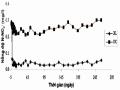 N-No2- Concentration (Mg/l) of Treatment Area and Control Area During the Test Period: (♦) Treatment Area, (■) Control Area.
 -
 Morphological Characteristics of K Lines (Winter-Spring Crop 2017-2018 in Gia Lam - Hanoi)

O(i,j) = O(i-1,j-1) + O(i-1,j) with 0 < j < i < n. For example, with n = 4, we have the table below:
Figure 6.1. Pascal's triangle rule O(n,k) is Comb(n,k) and we have the following algorithm:
Comb(n, k)
{
C[0][0] = 1;
for(i=1;i<=n;i++)
{
C[i][0] = 1;
C[i][i] = 1;
for(j=1;j<=i-1;j++)
C[i][j] =C[i-1][j-1] + C[i-1][j];
}
return(C[n][k])
}
The active operation is the operation C[i][j] =C[i-1][j-1] + C[i-1][j] whose time is
O(1). The for(j=1;j<=i-1;j++) loop executes i-1 times, each time O(1). The for(i=1;i<=n;i++) loop has i running from 1 to n, so if we call T(n) the algorithm execution time, we have:
n
T( n )
1
i 1 1 2 3 ... ( n 1 ) n( n 1 )
2
So T(n) = O(n 2 )
Comment :
Through determining the complexity, we can clearly see that the dynamic programming algorithm is much more efficient than the recursive algorithm (n 2 < 2 n ). However, using a table (two-dimensional array) as above is still a waste of memory cells, so we will improve it one step further by using a vector (one-dimensional array) to store intermediate results.
The specific steps are as follows:
We will use a vector V with n+1 elements from V[0] to V[n]. Vector V will store the values corresponding to row i in Pascal's triangle above. In which V[j] stores the value of the combination number j of i (j = 0 to i). Of course, because there is only one vector V, it must store many rows i, so at each step, V can only store one row and at the last step, V stores the values corresponding to i = n, in which V[k] is C k n .
Initially, for i = 1, we let V[0] = 1 and V[1] = 1. That is:
C
1
0 = 1 and
1
C 1= 1.
For values of i from 2 to n, we do the following:
i
- V[0] is assigned the value 1, that is C 0
= 1. However, the value V[0] = 1 has been
assigned above, no need to reassign.
i
- For j from 1 to i-1, we still apply the formula C j
j 1 i 1
j
C
i 1
. Means to
= C
To calculate the values in line i, we must rely on line i-1. However, since there is only one vector V and at this time it will store the values of line i, that is, line i-1 will no longer exist. To overcome this, we use two more intermediate variables p1 and p2. In which p1 is used to
i 1
i 1
i 1
C storagej 1 and p2 are used to store Cj . Initially p1 is assigned V[0] i.e. C 0 and
i 1
i
p2 is assigned V[j] i.e. C j , V[j] stores the value C j that will be assigned by p1+p2 , then
i 1
p1 is assigned by p2, meaning that when j increases by 1 to j+1 then p1 is C j
and it
i
is used to calculate C j 1 .
i
- Finally, with j = i, assign V[i] the value 1, that is, C i
= 1.
Solution:
Comb(n, k )
{
V[0] = 1;
V[1] = 1;
for(i=2;i<=n;i++)
{
p1 := V[0];
for(j=1;i<=i-1;j++)
{
p2 := V[j];
V[j]:= p1+p2; p1:= p2;
}
V[i] := 1;
}
return(V[k]);
}
It is easy to see that the complexity of the algorithm is still O(n 2 ).
6.2.2. Multiplication of multiple matrices
1) Problem
Calculate the product of the matrices: A = A 1 ×...× A n so that the number of calculations required is the least (Assuming that multiplications are possible ).
2) Problem analysis
We see that:
Due to the associative nature of matrix multiplication, matrices A i can be grouped in many different ways, without the resulting matrix A changing. However, there are differences in the cost of changing the combinations of matrices A i .
Below is the algorithm to multiply two matrices A and B, the attributes rows and columns are the number of rows and columns of the matrix.
MATRIX-MULTIPLY(A, B)
{
if ( columns[A] rows[B]) return;
else for(i=1;i<=rows[A];i++)
for(j=1;j<=columns[B];j++)
{
}
return C;
}
C[i, j] = 0
for(k=1;k<=columns[A];k++)
C[i, j] = C[i, j] + A[i, k] * B[k, j];
We can multiply two matrices A and B if and only if it is appropriate: the number of columns of matrix A must be equal to the number of rows of matrix B. If A is a matrix of size m n and B is an n p matrix, then the resulting matrix C has size m p. The time to compute C is determined by the number of operations C[i, j] = C[i, j] + A[i, k] * B[k, j], that is m n p.
To illustrate the difference in computing time C due to different placement of parentheses in matrix multiplication, consider matrices A, B, C, D with the following sizes:
A 30x1 B 1x40 C 40x10 D 10x25
Calculate the matrix product A × B × C × D
We will see that the cost of multiplying matrices depends on how the matrices are combined by multiplying them in different orders and calculating the cost in each way as follows:
Order
Expense | |
((AB)C)D | 30 × 1 × 40 + 30 × 40 × 10 + 30 × 10 × 25 = 20700 |
(A(B(CD)) | 40 × 10 × 25 + 1 × 40 × 25 + 30 × 1 × 25 = 11750 |
(AB)(CD) | 30 × 1 × 40 + 40 × 10 × 25 + 30 × 40 × 25 = 41200 |
A((BC)D) | 1 × 40 × 10 + 1 × 10 × 25 + 30 × 1 × 25 = 1400 |
Figure 6.2. Costs according to matrix combinations
3) Idea
We solve the problem using a bottom-up approach. We will calculate and store the optimal solution for each small part to avoid recomputing the larger problem.
First for sets of 2 matrices, sets of 3 matrices...
For example, to calculate A×B×C we can calculate in the following ways: (A×B)×C or A×(B×C).
So the cost to calculate A×B×C is the cost calculated from 2 parts:
Part one is the cost kq1×C, with kq1 = A×B (this cost has been calculated and saved).
storage)
The second part is the cost A × kq2, with kq2 = B×C (this cost has been stored) Compare the above 2 parts and store the smaller cost. . .
4) Algorithm design
The key is to compute the cost of multiplying sets of matrices: A i ×...×A j , with 1≤ i < j ≤ n, where smaller sets have already been computed and the results stored.
With a combination of matrices:
A i ×...×A j = (A i ×...×A k ) × (A k+1 ×...×A j )
The cost of multiplying matrices A i ,...,A j will be the sum of: Cost of multiplying A i ×...×A k ( kq1), cost of multiplying A k+1 ×...×A j ( kq2), and cost kq1×kq2.
then:
If M ij is called the minimum cost of multiplying the set of matrices A i ×...×A j ,1≤ i < j ≤ n
* M ik is the minimum cost to multiply the set of matrices A i ×...×A k
* M k+1,j is the minimum cost to multiply the set of matrices A k+1 ×...×A j With matrix kq1 of size d i-1 ×d k and kq2 of size d k ×d j , so the cost to multiply
kq1×kq2 is d i-1 d k d j .
Therefore:
M ij = Min {M ik + M k +1, j + d i −1 d k d j };1 ≤ i < j ≤ n
i ≤ k ≤ j −1
M ii = 0
We can consider M as an upper triangular matrix: (M ij )1≤i<j≤n . We need to calculate and fill the elements of this matrix until we determine M 1n . All elements on the main diagonal are 0.
To calculate M ij , we need to know M ik , M k+1,j . We calculate the table along the diagonals starting from the diagonal next to the main diagonal and moving towards the upper right corner.
We want to know the best order to multiply the array of matrices (in the sense of minimum cost). Each time we determine the best combination, we use a variable k to store this order. That is, O ij = k, for M ik + M k +1, j + d i −1 d k d j reaches min.
We store the M ij in a 2-dimensional array M.
The k indices to determine M ij are stored in a 2-dimensional array O.
The size of the matrices we store in a 1-dimensional array d : Ai is a matrix with d i-1 rows and d i columns.
Algorithm:
Input d = (d0,d1,...,dn); Output M = (Mij) ,
O = (Oij); MO(d,n,O,M)
{
for (i = 1; i <= n; i++) M[i][i] = 0;
for (diag = 1; diag <= n-1; diag++) for (i = 1; i <= n - diag; i++)
{
j = i + diag; csm = i;
min = M[i][i]+M[i+1][j]+d[i-1]*d[i]*d[j]; for (k= i; k <= j - 1; k++)
if (min > (M[i][k]+M[k+1][j]+d[i-1]*d[k]*d[j] ))
{
min= M[i][k]+M[k+1][j]+d[i-1]*d[k]*d[j]; csm = k;
}
M[i][j] = min;
O[i][j] = csm;
}
return M[1][n];
}
Then use the following function to output the order of matrix multiplication combinations: MOS(i, j, O)
{
if (i == j)
printf(Ai);
}
Example 6.1.
else
{
}
k = O[i][j];
printf("(");
MOS(i,k,O);
printf("*:);
MOS (k+1,j,O);
printf(")");
The algorithm is illustrated by matrix multiplication:
A 1 × A 2 × A 3 × A 4 × A 5 × A 6
With the sizes of the matrices being:
Matrix
Size | |
A 1 | 30 × 35 |
A 2 | 35 × 15 |
A 3 | 15 × 5 |
A 4 | 5 × 10 |
A 5 | 10 × 20 |
A 6 | 20 × 25 |
Figure 6.3. Size of the matrices
6
1
j
5
15,125
2
i
4 11,875 10,500
3
3
9,375
7.125
5.375
4
For convenience, we rotate arrays M and O so that the main diagonal is horizontal.
2 | 7,875 | 4,375 | 8,456 | 3,500 | 5 | |||
1 | 15,750 | 2,625 | 750 | 16,000 | 5,000 | 6 | ||
0 | 0 | 0 | 0 | 0 | 0 |
A 1 A 2 A 3 A 4 A 5 A 6
Figure 6.4. Array M
6
1
j
5
3
2
i
4
3
3
3
3
3
3
3
4
2
1
3
3
5
1
2
3
4
5
5
Figure 6.5. Array O