chosen experimentally by trial and error. A large value of α speeds up the convergence process. This is not always beneficial because if we assume from the beginning that the network converges quickly, it is very likely that the network will converge early at the nearest local minimum without achieving the desired error. However, setting the learning step value too small will cause the network to converge very slowly, or even bypass the local minima and thus lead to learning forever without converging. Figure 2.6 shows a function with contour lines that are stretched and curved to form a gap. For functions like this, how to choose the learning step so that it does not get stuck at the gap axis?
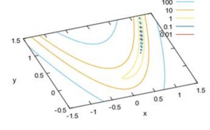
Figure 2.6: Slot contour lines
In this section, the author presents a gap crossing technique to be applied to find the optimal weight set of the network. Then, we will use a simple example to show that the steepest descent backpropagation (SDBP) technique has problems with convergence and the author will present the combination of the gap crossing algorithm and the backpropagation technique to improve the convergence of the solution.
Figure 2.7 shows the training algorithm of MLP neural network using back propagation learning with gap-crossing step. The algorithm for calculating the gap-crossing step is shown in Figure 2.4 .
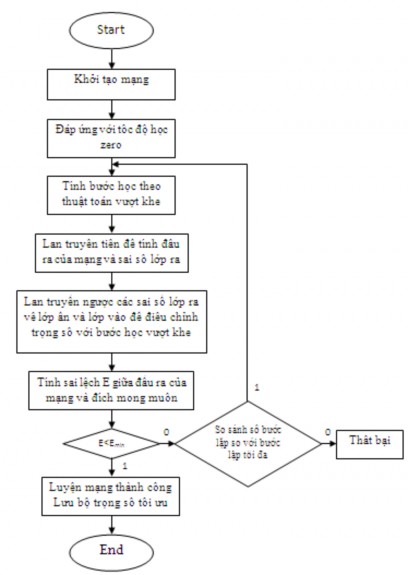
Figure 2.7: Flowchart of MLP neural network training algorithm with gap-pass learning step
2.3. Algorithm illustration
An example problem to illustrate the training algorithm with gap-pass learning is as follows: Given an input vector to the network input, the neural network must tell us what the input is.
2.3.1. Preparation work
Objective: successfully implement a neural network training method using the back propagation procedure combined with a learning step calculated according to the gap-crossing principle to find the global optimal solution for the error surface in the form of a gap.
Using the fastest descent method to update the weights of the network, we need information regarding the partial derivatives of the error function taken over each weight, which means that our remaining problem in the preparation work is to present the formulas and algorithms for updating the weights in the hidden and output layers.
Given a set of samples, we will calculate the derivative of the error function by taking the sum of the derivatives of the error function over each sample in that set. This method of analysis and calculation of derivatives is based on the “chain rule”.
For a single-layer linear network (ADLINE), the partial derivatives are conveniently calculated. For a multilayer network, the error is not an explicit function of the weights in the hidden layers, so we use the chain rule to calculate the derivatives. The slope of the tangent to the error curve in the cross-section along the w axis is called the partial derivative of the error function J with respect to that weight, denoted by J/ w, using the rule
J J w w
series we have .1...n
w w w w
1 2
2.3.1.1. Adjust the output layer weights
Call: b: output layer weight
z: output of the output layer neuron. t: desired target value
y j : output of the neuron in the hidden layer
v: sum of weights
output layer neurons)
M 1
v b j y j should v/ b j = y j (ignoring the indices of the
j 0
We use J = 0.5*(zt) 2 , so J/ z = (zt).
The activation function of the output layer neuron is sigmoid z=g(v), with z/ v = z(1-z).
We have:
J J . z . v z t . z 1 z . y
(2.16)
b z v b
From there we have the following formula to update the class weights (ignoring the indices):
PhD Thesis in Engineering
2013
b . z t . z . 1 z . y
(2.17)
We will use formula (2.17) [21] in the DIEUCHINHTRONGSO() procedure to adjust the output layer weights, in which there is an emphasis that the learning rate α is calculated according to the gap-crossing principle, which is the goal of the study.
void DIEUCHINHTRONGSO(int k)
{
int i,j; float temp;
SAISODAURA(); for(i=0;i<SLNRLA;i++)
{
for(j=0;j<SLNRLR;j++)
{
temp = -TOCDOHOC*y[i]*z[j]*(1-z[j])*SSLR[j]; MTTSLR[i][j] = MTTSLR[i][j] + temp + QUANTINH*BTMTTSLR[i][j];
BTMTTSLR[i][j] = temp;
}
}
}
2.3.1.2. Adjust hidden layer weights
The derivative of the network's objective function with respect to a hidden layer weight is given by
chain rule, J
a J
y . y
u . u
a .
Call: a: hidden layer weight
y: output of a neuron in the hidden layer
x i : components of the input vector of the input layer
N 1
u: weighted sum u a i x i should u/ a i = x i
i 0
k: index of neurons in output layer
Hidden layers do not cause errors by themselves, but they contribute to the error of the model.
class out. We have
J K 1 J
y z
z k
v
v k
yes
k 0 k
We only consider one hidden layer neuron, so we omit the hidden layer index for simplicity. Here we see that the quantity J z . z v is propagated back to the hidden layer,
k index says that
J z
z k v
z k t k . z k . 1 z k
(This formula is
k k
from section 3.1.1) belongs to which neuron in the output layer. As we know, v is the sum of the weights
chemical, so v y b , with index k we have
v k b . Here, the first term
yes
belong to J a J y . y u . u a
has been completed.
J
K 1
z
t . z . 1 z . b
, in this formula we have omitted the index of
yes
k 0
kkkkk
The hidden layer neuron, which is associated with y (written in full should be
J y
, with j=0...M-1).
i
Next, we consider the second term y u , which describes the change of the input.
output of a neuron in the hidden layer according to the weighted sum of the input vector components of the input layer. We have the relationship between y and u according to the neuron activation function
y 1 1 e u , so y
u y . 1 y . The remaining third term u
a is the
transformation of the output of the hidden layer neuron according to the hidden layer weights. Since u is the weighted sum of
N 1
input vector components
u a i x i
i 0
so we have immediately u
a i x i . In summary,
We have the derivative of the objective function with respect to a weight of the hidden layer:
JK 1 z
t . z . 1 z . b . y . 1 y . x
(2.18)
a
kkkkki
ik 0
From here we come to the formula for adjusting the weights for the hidden layer:
K 1
a i . z kt k . z k . 1 z k . b k . y . 1 y . x i
k 0
(2.19)
In formula (2.19) the index i represents the i-th neuron of the input layer, the index k represents the k-th neuron of the output layer; in the formula we did not represent the index j, the index represents the hidden layer neuron.
We will use formula (2.19) [21] in the procedure DIEUCHINHTRONGSO()
To adjust the hidden layer weights, the learning rate α is calculated using the gap crossing principle.
The DIEUCHINHTRONGSO() procedure code is presented as follows, in which the float variable temp is the weight variation value and the temp variable is calculated according to formula (2.19). (A part of formula (2.19) is calculated in the SAISOLOPAN() procedure .)
void DIEUCHINHTRONGSO(int k)
{
int i,j; float temp;
SAISOLOPAN(); for(i=0;i<SLNRLV;i++)
{
for(j=0;j<SLNRLA;j++)
{
temp = -TOCDOHOC*x[i]*y[j]*(1-y[j])*SSLA[j]; MTTSLA[i][j] = MTTSLA[i][j] + temp +
QUANTINH*BTMTTSLA[i][j];
BTMTTSLA[i][j] = temp;
}
}
}
2.3.2. Network structure
From the information obtained from sections 2.3 and 2.1, together with the requirements of the example problem stated in section 1.4.2., it is necessary to recognize the characters as digits 0, 1, .., 9.
In addition, the author also gives another example of recognizing the letters: a, b, c, d, e, g, h, i, k, l.
Figure 1.5 describes the structure of a multilayer neural network with 35 input neurons, 5 hidden neurons and 10 output neurons; the function f is chosen to be sigmoid.
1
f 1 exp -x
We also say a few words about the use of bias. Neurons may or may not have biases. Bias allows the network to adjust and strengthen the network. Sometimes we want to avoid the argument of the function f being zero when all the inputs to the network are zero, the bias coefficient will do the job of avoiding the sum of the weights being zero. In the network structure of Figure 1.5, we ignore the participation of biases. Some further discussion about how to choose an optimal network structure for our problem is not yet resolved, here we only do this well based on trial and error. Next, what happens if we design a network that needs to have more than two layers? How many neurons in the hidden layer will it be? This problem sometimes has to be predicted in advance or can also be through research and experimentation. Whether a neural network is good or not, the first thing to do is to choose a good network structure. Specifically, we will choose which activation function (transfer function) from a series of available functions (see table 2.1). We can also build our own activation function for our problem without using those available functions. Suppose, the preliminary selection of a network structure as shown in figure 1.5 is complete. We will start the network training work, that is, adjusting the network's numbers (w). If after a training effort we do not achieve the optimal numbers (w*), then the network structure we chose may have problems, of course, we have to do this work again from the beginning, that is, choose another network structure, and train again... After the network training process, we may encounter the problem that some neurons in the network do not participate in the work of the problem at all, which is shown in the weight coefficients w connected to that neuron being close to zero. Of course, we will remove that neuron to optimize the memory and running time of the network.
2.3.3. Network libraries and functions
Table 2.1. Typical transfer functions [6]
Function name
Function description | Icon | Matlab Function | |
Hard Limit | f 0 if x 0 1 if x 0 |
| Hardlim |
Symmetrical Hard Limit | f 1 if x 0 1 if x 0 |
| Hardlims |
Linear | f x |
| Purelin |
Log-sigmoid | f 1 1 exp -x |
| logsig |


Maybe you are interested!
-

 Organizing Workshops, Training and Lectures to Disseminate and Share Network Resources and Teaching Methods Using IT
 -
 Neural Network Coordination for ECG Signal Recognition Using Decision Tree Model
 -
 Wireless Network Technology Network Administration Profession - Vocational College - General Department of Vocational Training - 7
 -
 Borrowing, Dynamic Channel Locking Based on Fuzzy Logic Controller and Neural Network
 -
 Training and Professional Development of Land Price Management Team
2.3.3.1. Library
In the dinhnghia.h file, the sigmoid function is stated along with its derivative, which is characterized by being very flat for large inputs, thus easily generating a narrow canyon-shaped quality surface. So the question arises, is it mandatory for all neurons in a layer to have the same activation functions? The answer is no, we can define a layer of neurons with different activation functions. We use the activation function that is commonly used in neural network techniques, the sigmoid function for all neurons in the network.
#define SIGMF(x) 1/(1 + exp(-(double)x))
#define DSIGM(y) (float)(y)*(1.0-y))
The number of input neurons of the network is equal to the number of components of the input vector x with size 35×1.
#define SLNRLV 35 // SO LUONG NO RON LOP VAO
The number of hidden layer neurons is 5, the hidden layer output response vector is y with size 5×1. It can be said that there is no work that specifically talks about the size of the hidden layer. However, if you choose a hidden layer size that is too large, it is not recommended for the problems.