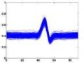
Extract the results of the QRS complex detection algorithm, tested with 100 records in the MIT-BIH database set, the results are shown in Figure 3.6-f.
(a)
(b)
(c)
(d)
(e)
(f)
Figure 3.6. Example steps of R peak detection: (a) original ECG signal, (b) filtered result,
(c) result after taking derivative, (d) result after taking absolute value, (e) result after taking average, (f) result of detecting R peak.
3.1.2. Analysis of QRS complex by basis Hermite functions
Analyzing the ECG signal by Hermite function is a quite popular method, has been used by many authors, the results are good and this method is also chosen for the thesis. In this section, the author will present the process of creating characteristic vectors of the ECG signal.
a) Hermite function
The Hermite polynomial is given in recursive form by the following formula:
H n 1 ( x ) 2 x H n ( x ) 2 n H n 1 ( x )
(3.6)
give
n 1,
with
H 0 ( x ) 1; H 1 ( x ) 2 x .
The Hermite function is defined by the following formula:
n ( x )
2 n n ! 2e
x 2
2 H n ( x )
1
(3.7)
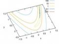
Some shapes of Hermite functions are shown in Figure 3.7. We can see that the higher the degree of the Hermite function, the greater the rate of change of the function, or in other words, the function will contain more high-order components. At the same time, the shape of the functions is quite similar to the shape of the basic components in the ECG signal. This is the basis for using Hermite functions to analyze electrocardiogram signals.
-5 | 0 | 5 | 10 -10 | -5 | 0 | 5 | 10 | |
(c) | (d) |
Maybe you are interested!
-
 Description of the Mlp Neural Network Training Algorithm Using Backpropagation Learning with Overshoot Step. Algorithm for Calculating Overshoot Step
 -
 Quality Evaluation Criteria of ECG Signal Recognition Model
 -
 Borrowing, Dynamic Channel Locking Based on Fuzzy Logic Controller and Neural Network
 -
![Qos Assurance Methods for Multimedia Communications
zt2i3t4l5ee
zt2a3gs
zt2a3ge
zc2o3n4t5e6n7ts
low. The EF PHB requires a sufficiently large number of output ports to provide low delay, low loss, and low jitter.
EF PHBs can be implemented if the output ports bandwidth is sufficiently large, combined with small buffer sizes and other network resources dedicated to EF packets, to allow the routers service rate for EF packets on an output port to exceed the arrival rate λ of packets at that port.
This means that packets with PHB EF are considered with a pre-allocated amount of output bandwidth and a priority that ensures minimum loss, minimum delay and minimum jitter before being put into operation.
PHB EF is suitable for channel simulation, leased line simulation, and real-time services such as voice, video without compromising on high loss, delay and jitter values.
Figure 2.10 Example of EF installation
Figure 2.10 shows an example of an EF PHB implementation. This is a simple priority queue scheduling technique. At the edges of the DS domain, EF packet traffic is prioritized according to the values agreed upon by the SLA. The EF queue in the figure needs to output packets at a rate higher than the packet arrival rate λ. To provide an EF PHB over an end-to-end DS domain, bandwidth at the output ports of the core routers needs to be allocated in advance to ensure the requirement μ > λ. This can be done by a pre-configured provisioning process. In the figure, EF packets are placed in the priority queue (the upper queue). With such a length, the queue can operate with μ > λ.
Since EF was primarily used for real-time services such as voice and video, and since real-time services use UDP instead of TCP, RED is generally
not suitable for EF queues because applications using UDP will not respond to random packet drop and RED will strip unnecessary packets.
2.2.4.2 Assured Forwarding (AF) PHB
PHB AF is defined by RFC 2597. The purpose of PHB AF is to deliver packets reliably and therefore delay and jitter are considered less important than packet loss. PHB AF is suitable for non-real-time services such as applications using TCP. PHB AF first defines four classes: AF1, AF2, AF3, AF4. For each of these AF classes, packets are then classified into three subclasses with three distinct priority levels.
Table 2.8 shows the four AF classes and 12 AF subclasses and the DSCP values for the 12 AF subclasses defined by RFC 2597. RFC 2597 also allows for more than three separate priority levels to be added for internal use. However, these separate priority levels will only have internal significance.
PHB Class
PHB Subclass
Package type
DSCP
AF4
AF41
Short
100010
AF42
Medium
100100
AF43
High
100110
AF3
AF31
Short
011010
AF32
Medium
011100
AF33
High
011110
AF2
AF21
Short
010010
AF22
Medium
010100
AF23
High
010110
AF1
AF11
Short
001010
AF12
Medium
001100
AF13
High
001110
Table 2.8 AF DSCPs
The AF PHB ensures that packets are forwarded with a high probability of delivery to the destination within the bounds of the rate agreed upon in an SLA. If AF traffic at an ingress port exceeds the pre-priority rate, which is considered non-compliant or “out of profile”, the excess packets will not be delivered to the destination with the same probability as the packets belonging to the defined traffic or “in profile” packets. When there is network congestion, the out of profile packets are dropped before the in profile packets are dropped.
When service levels are defined using AF classes, different quantity and quality between AF classes can be realized by allocating different amounts of bandwidth and buffer space to the four AF classes. Unlike
EF, most AF traffic is non-real-time traffic using TCP, and the RED queue management strategy is an AQM (Adaptive Queue Management) strategy suitable for use in AF PHBs. The four AF PHB layers can be implemented as four separate queues. The output port bandwidth is divided into four AF queues. For each AF queue, packets are marked with three “colors” corresponding to three separate priority levels.
In addition to the 32 DSCP 1 groups defined in Table 2.8, 21 DSCPs have been standardized as follows: one for PHB EF, 12 for PHB AF, and 8 for CSCP. There are 11 DSCP 1 groups still available for other standards.
2.2.5.Example of Differentiated Services
We will look at an example of the Differentiated Service model and mechanism of operation. The architecture of Differentiated Service consists of two basic sets of functions:
Edge functions: include packet classification and traffic conditioning. At the inbound edge of the network, incoming packets are marked. In particular, the DS field in the packet header is set to a certain value. For example, in Figure 2.12, packets sent from H1 to H3 are marked at R1, while packets from H2 to H4 are marked at R2. The labels on the received packets identify the service class to which they belong. Different traffic classes receive different services in the core network. The RFC definition uses the term behavior aggregate rather than the term traffic class. After being marked, a packet can be forwarded immediately into the network, delayed for a period of time before being forwarded, or dropped. We will see that there are many factors that affect how a packet is marked, and whether it is forwarded immediately, delayed, or dropped.
Figure 2.12 DiffServ Example
Core functionality: When a DS-marked packet arrives at a Diffservcapable router, the packet is forwarded to the next router based on
Per-hop behavior is associated with packet classes. Per-hop behavior affects router buffers and the bandwidth shared between competing classes. An important principle of the Differentiated Service architecture is that a routers per-hop behavior is based only on the packets marking or the class to which it belongs. Therefore, if packets sent from H1 to H3 as shown in the figure receive the same marking as packets from H2 to H4, then the network routers treat the packets exactly the same, regardless of whether the packet originated from H1 or H2. For example, R3 does not distinguish between packets from h1 and H2 when forwarding packets to R4. Therefore, the Differentiated Service architecture avoids the need to maintain router state about separate source-destination pairs, which is important for network scalability.
Chapter Conclusion
Chapter 2 has presented and clarified two main models of deploying and installing quality of service in IP networks. While the traditional best-effort model has many disadvantages, later models such as IntServ and DiffServ have partly solved the problems that best-effort could not solve. IntServ follows the direction of ensuring quality of service for each separate flow, it is built similar to the circuit switching model with the use of the RSVP resource reservation protocol. IntSer is suitable for services that require fixed bandwidth that is not shared such as VoIP services, multicast TV services. However, IntSer has disadvantages such as using a lot of network resources, low scalability and lack of flexibility. DiffServ was born with the idea of solving the disadvantages of the IntServ model.
DiffServ follows the direction of ensuring quality based on the principle of hop-by-hop behavior based on the priority of marked packets. The policy for different types of traffic is decided by the administrator and can be changed according to reality, so it is very flexible. DiffServ makes better use of network resources, avoiding idle bandwidth and processing capacity on routers. In addition, the DifServ model can be deployed on many independent domains, so the ability to expand the network becomes easy.
Chapter 3: METHODS TO ENSURE QoS FOR MULTIMEDIA COMMUNICATIONS
In packet-switched networks, different packet flows often have to share the transmission medium all the way to the destination station. To ensure the fair and efficient allocation of bandwidth to flows, appropriate serving mechanisms are required at network nodes, especially at gateways or routers, where many different data flows often pass through. The scheduler is responsible for serving packets of the selected flow and deciding which packet will be served next. Here, a flow is understood as a set of packets belonging to the same priority class, or originating from the same source, or having the same source and destination addresses, etc.
In normal state when there is no congestion, packets will be sent as soon as they are delivered. In case of congestion, if QoS assurance methods are not applied, prolonged congestion can cause packet drops, affecting service quality. In some cases, congestion is prolonged and widespread in the network, which can easily lead to the network being frozen, or many packets being dropped, seriously affecting service quality.
Therefore, in this chapter, in sections 3.2 and 3.3, we introduce some typical network traffic load monitoring techniques to predict and prevent congestion before it occurs through the measure of dropping (removing) packets early when there are signs of impending congestion.
3.1. DropTail method
DropTail is a simple, traditional queue management method based on FIFO mechanism. All incoming packets are placed in the queue, when the queue is full, the later packets are dropped.
Due to its simplicity and ease of implementation, DropTail has been used for many years on Internet router systems. However, this algorithm has the following disadvantages:
− Cannot avoid the phenomenon of “Lock out”: Occurs when 1 or several traffic streams monopolize the queue, making packets of other connections unable to pass through the router. This phenomenon greatly affects reliable transmission protocols such as TCP. According to the anti-congestion algorithm, when locked out, the TCP connection stream will reduce the window size and reduce the packet transmission speed exponentially.
− Can cause Global Synchronization: This is the result of a severe “Lock out” phenomenon. Some neighboring routers have their queues monopolized by a number of connections, causing a series of other TCP connections to be unable to pass through and simultaneously reducing the transmission speed. After those monopolized connections are temporarily suspended,
Once the queue is cleared, it takes a considerable amount of time for TCP connections to return to their original speed.
− Full Queue phenomenon: Data transmitted on the Internet often has an explosion, packets arriving at the router are often in clusters rather than in turn. Therefore, the operating mechanism of DropTail makes the queue easily full for a long period of time, leading to the average delay time of large packets. To avoid this phenomenon, with DropTail, the only way is to increase the routers buffer, this method is very expensive and ineffective.
− No QoS guarantee: With the DropTail mechanism, there is no way to prioritize important packets to be transmitted through the router earlier when all are in the queue. Meanwhile, with multimedia communication, ensuring connection and stable speed is extremely important and the DropTail algorithm cannot satisfy.
The problem of choosing the buffer size of the routers in the network is to “absorb” short bursts of traffic without causing too much queuing delay. This is necessary in bursty data transmission. The queue size determines the size of the packet bursts (traffic spikes) that we want to be able to transmit without being dropped at the routers.
In IP-based application networks, packet dropping is an important mechanism for indirectly reporting congestion to end stations. A solution that prevents router queues from filling up while reducing the packet drop rate is called dynamic queue management.
3.2. Random elimination method – RED
3.2.1 Overview
RED (Random Early Detection of congestion; Random Early Drop) is one of the first AQM algorithms proposed in 1993 by Sally Floyd and Van Jacobson, two scientists at the Lawrence Berkeley Laboratory of the University of California, USA. Due to its outstanding advantages compared to previous queue management algorithms, RED has been widely installed and deployed on the Internet.
The most fundamental point of their work is that the most effective place to detect congestion and react to it is at the gateway or router.
Source entities (senders) can also do this by estimating end-to-end delay, throughput variability, or the rate of packet retransmissions due to drop. However, the sender and receiver view of a particular connection cannot tell which gateways on the network are congested, and cannot distinguish between propagation delay and queuing delay. Only the gateway has a true view of the state of the queue, the link share of the connections passing through it at any given time, and the quality of service requirements of the
traffic flows. The RED gateway monitors the average queue length, which detects early signs of impending congestion (average queue length exceeding a predetermined threshold) and reacts appropriately in one of two ways:
− Drop incoming packets with a certain probability, to indirectly inform the source of congestion, the source needs to reduce the transmission rate to keep the queue from filling up, maintaining the ability to absorb incoming traffic spikes.
− Mark “congestion” with a certain probability in the ECN field in the header of TCP packets to notify the source (the receiving entity will copy this bit into the acknowledgement packet).
Figure 3. 1 RED algorithm
The main goal of RED is to avoid congestion by keeping the average queue size within a sufficiently small and stable region, which also means keeping the queuing delay sufficiently small and stable. Achieving this goal also helps: avoid global synchronization, not resist bursty traffic flows (i.e. flows with low average throughput but high volatility), and maintain an upper bound on the average queue size even in the absence of cooperation from transport layer protocols.
To achieve the above goals, RED gateways must do the following:
− The first is to detect congestion early and react appropriately to keep the average queue size small enough to keep the network operating in the low latency, high throughput region, while still allowing the queue size to fluctuate within a certain range to absorb short-term fluctuations. As discussed above, the gateway is the most appropriate place to detect congestion and is also the most appropriate place to decide which specific connection to report congestion to.
− The second thing is to notify the source of congestion. This is done by marking and notifying the source to reduce traffic. Normally the RED gateway will randomly drop packets. However, if congestion
If congestion is detected before the queue is full, it should be combined with packet marking to signal congestion. The RED gateway has two options: drop or mark; where marking is done by marking the ECN field of the packet with a certain probability, to signal the source to reduce the traffic entering the network.
− An important goal that RED gateways need to achieve is to avoid global synchronization and not to resist traffic flows that have a sudden characteristic. Global synchronization occurs when all connections simultaneously reduce their transmission window size, leading to a severe drop in throughput at the same time. On the other hand, Drop Tail or Random Drop strategies are very sensitive to sudden flows; that is, the gateway queue will often overflow when packets from these flows arrive. To avoid these two phenomena, gateways can use special algorithms to detect congestion and decide which connections will be notified of congestion at the gateway. The RED gateway randomly selects incoming packets to mark; with this method, the probability of marking a packet from a particular connection is proportional to the connections shared bandwidth at the gateway.
− Another goal is to control the average queue size even without cooperation from the source entities. This can be done by dropping packets when the average size exceeds an upper threshold (instead of marking it). This approach is necessary in cases where most connections have transmission times that are less than the round-trip time, or where the source entities are not able to reduce traffic in response to marking or dropping packets (such as UDP flows).
3.2.2 Algorithm
This section describes the algorithm for RED gateways. RED gateways calculate the average queue size using a low-pass filter. This average queue size is compared with two thresholds: minth and maxth. When the average queue size is less than the lower threshold, no incoming packets are marked or dropped; when the average queue size is greater than the upper threshold, all incoming packets are dropped. When the average queue size is between minth and maxth, each incoming packet is marked or dropped with a probability pa, where pa is a function of the average queue size avg; the probability of marking or dropping a packet for a particular connection is proportional to the bandwidth share of that connection at the gateway. The general algorithm for a RED gateway is described as follows: [5]
For each packet arrival
Caculate the average queue size avg If minth ≤ avg < maxth
div.maincontent .s1 { color: black; font-family:Times New Roman, serif; font-style: normal; font-weight: normal; text-decoration: none; font-size: 15pt; }
div.maincontent .s2 { color: black; font-family:Times New Roman, serif; font-style: normal; font-weight: bold; text-decoration: none; font-size: 15pt; }
div.maincontent .p { color: black; font-family:Times New Roman, serif; font-style: normal; font-weight: normal; text-decoration: none; font-size: 14pt; margin:0pt; }
div.maincontent p { color: black; font-family:Times New Roman, serif; font-style: normal; font-weight: normal; text-decoration: none; font-size: 14pt; margin:0pt; }
div.maincontent .s3 { color: black; font-family:Times New Roman, serif; font-style: normal; font-weight: bold; text-decoration: none; font-size: 14pt; }
div.maincontent .s4 { color: black; font-family:Times New Roman, serif; font-style: normal; font-weight: normal; text-decoration: none; font-size: 14pt; }
div.maincontent .s5 { color: black; font-family:Times New Roman, serif; font-style: italic; font-weight: normal; text-decoration: none; font-size: 14pt; }
div.maincontent .s6 { color: black; font-family:Times New Roman, serif; font-style: italic; font-weight: bold; text-decoration: none; font-size: 14pt; }
div.maincontent .s7 { color: black; font-family:Wingdings; font-style: normal; font-weight: normal; text-decoration: none; font-size: 14pt; }
div.maincontent .s8 { color: black; font-family:Arial, sans-serif; font-style: italic; font-weight: bold; text-decoration: none; font-size: 15pt; }
div.maincontent .s9 { color: black; font-family:Times New Roman, serif; font-style: normal; font-weight: bold; text-decoration: none; font-size: 14pt; }
div.maincontent .s10 { color: black; font-family:Times New Roman, serif; font-style: normal; font-weight: normal; text-decoration: none; font-size: 9pt; vertical-align: 6pt; }
div.maincontent .s11 { color: black; font-family:Times New Roman, serif; font-style: normal; font-weight: normal; text-decoration: none; font-size: 13pt; }
div.maincontent .s12 { color: black; font-family:Times New Roman, serif; font-style: normal; font-weight: normal; text-decoration: none; font-size: 10pt; }
div.maincontent .s13 { color: black; font-family:Times New Roman, serif; font-style: normal; font-weight: normal; text-d](https://tailieuthamkhao.com/uploads/2022/05/15/danh-gia-hieu-qua-dam-bao-qos-cho-truyen-thong-da-phuong-tien-cua-chien-6-1-120x90.jpg) Qos Assurance Methods for Multimedia Communications
zt2i3t4l5ee
zt2a3gs
zt2a3ge
zc2o3n4t5e6n7ts
low. The EF PHB requires a sufficiently large number of output ports to provide low delay, low loss, and low jitter.
EF PHBs can be implemented if the output port's bandwidth is sufficiently large, combined with small buffer sizes and other network resources dedicated to EF packets, to allow the router's service rate for EF packets on an output port to exceed the arrival rate λ of packets at that port.
This means that packets with PHB EF are considered with a pre-allocated amount of output bandwidth and a priority that ensures minimum loss, minimum delay and minimum jitter before being put into operation.
PHB EF is suitable for channel simulation, leased line simulation, and real-time services such as voice, video without compromising on high loss, delay and jitter values.
Figure 2.10 Example of EF installation
Figure 2.10 shows an example of an EF PHB implementation. This is a simple priority queue scheduling technique. At the edges of the DS domain, EF packet traffic is prioritized according to the values agreed upon by the SLA. The EF queue in the figure needs to output packets at a rate higher than the packet arrival rate λ. To provide an EF PHB over an end-to-end DS domain, bandwidth at the output ports of the core routers needs to be allocated in advance to ensure the requirement μ > λ. This can be done by a pre-configured provisioning process. In the figure, EF packets are placed in the priority queue (the upper queue). With such a length, the queue can operate with μ > λ.
Since EF was primarily used for real-time services such as voice and video, and since real-time services use UDP instead of TCP, RED is generally
not suitable for EF queues because applications using UDP will not respond to random packet drop and RED will strip unnecessary packets.
2.2.4.2 Assured Forwarding (AF) PHB
PHB AF is defined by RFC 2597. The purpose of PHB AF is to deliver packets reliably and therefore delay and jitter are considered less important than packet loss. PHB AF is suitable for non-real-time services such as applications using TCP. PHB AF first defines four classes: AF1, AF2, AF3, AF4. For each of these AF classes, packets are then classified into three subclasses with three distinct priority levels.
Table 2.8 shows the four AF classes and 12 AF subclasses and the DSCP values for the 12 AF subclasses defined by RFC 2597. RFC 2597 also allows for more than three separate priority levels to be added for internal use. However, these separate priority levels will only have internal significance.
PHB Class
PHB Subclass
Package type
DSCP
AF4
AF41
Short
100010
AF42
Medium
100100
AF43
High
100110
AF3
AF31
Short
011010
AF32
Medium
011100
AF33
High
011110
AF2
AF21
Short
010010
AF22
Medium
010100
AF23
High
010110
AF1
AF11
Short
001010
AF12
Medium
001100
AF13
High
001110
Table 2.8 AF DSCPs
The AF PHB ensures that packets are forwarded with a high probability of delivery to the destination within the bounds of the rate agreed upon in an SLA. If AF traffic at an ingress port exceeds the pre-priority rate, which is considered non-compliant or “out of profile”, the excess packets will not be delivered to the destination with the same probability as the packets belonging to the defined traffic or “in profile” packets. When there is network congestion, the out of profile packets are dropped before the in profile packets are dropped.
When service levels are defined using AF classes, different quantity and quality between AF classes can be realized by allocating different amounts of bandwidth and buffer space to the four AF classes. Unlike
EF, most AF traffic is non-real-time traffic using TCP, and the RED queue management strategy is an AQM (Adaptive Queue Management) strategy suitable for use in AF PHBs. The four AF PHB layers can be implemented as four separate queues. The output port bandwidth is divided into four AF queues. For each AF queue, packets are marked with three “colors” corresponding to three separate priority levels.
In addition to the 32 DSCP 1 groups defined in Table 2.8, 21 DSCPs have been standardized as follows: one for PHB EF, 12 for PHB AF, and 8 for CSCP. There are 11 DSCP 1 groups still available for other standards.
2.2.5.Example of Differentiated Services
We will look at an example of the Differentiated Service model and mechanism of operation. The architecture of Differentiated Service consists of two basic sets of functions:
Edge functions: include packet classification and traffic conditioning. At the inbound edge of the network, incoming packets are marked. In particular, the DS field in the packet header is set to a certain value. For example, in Figure 2.12, packets sent from H1 to H3 are marked at R1, while packets from H2 to H4 are marked at R2. The labels on the received packets identify the service class to which they belong. Different traffic classes receive different services in the core network. The RFC definition uses the term behavior aggregate rather than the term traffic class. After being marked, a packet can be forwarded immediately into the network, delayed for a period of time before being forwarded, or dropped. We will see that there are many factors that affect how a packet is marked, and whether it is forwarded immediately, delayed, or dropped.
Figure 2.12 DiffServ Example
Core functionality: When a DS-marked packet arrives at a Diffservcapable router, the packet is forwarded to the next router based on
Per-hop behavior is associated with packet classes. Per-hop behavior affects router buffers and the bandwidth shared between competing classes. An important principle of the Differentiated Service architecture is that a router's per-hop behavior is based only on the packet's marking or the class to which it belongs. Therefore, if packets sent from H1 to H3 as shown in the figure receive the same marking as packets from H2 to H4, then the network routers treat the packets exactly the same, regardless of whether the packet originated from H1 or H2. For example, R3 does not distinguish between packets from h1 and H2 when forwarding packets to R4. Therefore, the Differentiated Service architecture avoids the need to maintain router state about separate source-destination pairs, which is important for network scalability.
Chapter Conclusion
Chapter 2 has presented and clarified two main models of deploying and installing quality of service in IP networks. While the traditional best-effort model has many disadvantages, later models such as IntServ and DiffServ have partly solved the problems that best-effort could not solve. IntServ follows the direction of ensuring quality of service for each separate flow, it is built similar to the circuit switching model with the use of the RSVP resource reservation protocol. IntSer is suitable for services that require fixed bandwidth that is not shared such as VoIP services, multicast TV services. However, IntSer has disadvantages such as using a lot of network resources, low scalability and lack of flexibility. DiffServ was born with the idea of solving the disadvantages of the IntServ model.
DiffServ follows the direction of ensuring quality based on the principle of hop-by-hop behavior based on the priority of marked packets. The policy for different types of traffic is decided by the administrator and can be changed according to reality, so it is very flexible. DiffServ makes better use of network resources, avoiding idle bandwidth and processing capacity on routers. In addition, the DifServ model can be deployed on many independent domains, so the ability to expand the network becomes easy.
Chapter 3: METHODS TO ENSURE QoS FOR MULTIMEDIA COMMUNICATIONS
In packet-switched networks, different packet flows often have to share the transmission medium all the way to the destination station. To ensure the fair and efficient allocation of bandwidth to flows, appropriate serving mechanisms are required at network nodes, especially at gateways or routers, where many different data flows often pass through. The scheduler is responsible for serving packets of the selected flow and deciding which packet will be served next. Here, a flow is understood as a set of packets belonging to the same priority class, or originating from the same source, or having the same source and destination addresses, etc.
In normal state when there is no congestion, packets will be sent as soon as they are delivered. In case of congestion, if QoS assurance methods are not applied, prolonged congestion can cause packet drops, affecting service quality. In some cases, congestion is prolonged and widespread in the network, which can easily lead to the network being "frozen", or many packets being dropped, seriously affecting service quality.
Therefore, in this chapter, in sections 3.2 and 3.3, we introduce some typical network traffic load monitoring techniques to predict and prevent congestion before it occurs through the measure of dropping (removing) packets early when there are signs of impending congestion.
3.1. DropTail method
DropTail is a simple, traditional queue management method based on FIFO mechanism. All incoming packets are placed in the queue, when the queue is full, the later packets are dropped.
Due to its simplicity and ease of implementation, DropTail has been used for many years on Internet router systems. However, this algorithm has the following disadvantages:
− Cannot avoid the phenomenon of “Lock out”: Occurs when 1 or several traffic streams monopolize the queue, making packets of other connections unable to pass through the router. This phenomenon greatly affects reliable transmission protocols such as TCP. According to the anti-congestion algorithm, when locked out, the TCP connection stream will reduce the window size and reduce the packet transmission speed exponentially.
− Can cause Global Synchronization: This is the result of a severe “Lock out” phenomenon. Some neighboring routers have their queues monopolized by a number of connections, causing a series of other TCP connections to be unable to pass through and simultaneously reducing the transmission speed. After those monopolized connections are temporarily suspended,
Once the queue is cleared, it takes a considerable amount of time for TCP connections to return to their original speed.
− Full Queue phenomenon: Data transmitted on the Internet often has an explosion, packets arriving at the router are often in clusters rather than in turn. Therefore, the operating mechanism of DropTail makes the queue easily full for a long period of time, leading to the average delay time of large packets. To avoid this phenomenon, with DropTail, the only way is to increase the router's buffer, this method is very expensive and ineffective.
− No QoS guarantee: With the DropTail mechanism, there is no way to prioritize important packets to be transmitted through the router earlier when all are in the queue. Meanwhile, with multimedia communication, ensuring connection and stable speed is extremely important and the DropTail algorithm cannot satisfy.
The problem of choosing the buffer size of the routers in the network is to “absorb” short bursts of traffic without causing too much queuing delay. This is necessary in bursty data transmission. The queue size determines the size of the packet bursts (traffic spikes) that we want to be able to transmit without being dropped at the routers.
In IP-based application networks, packet dropping is an important mechanism for indirectly reporting congestion to end stations. A solution that prevents router queues from filling up while reducing the packet drop rate is called dynamic queue management.
3.2. Random elimination method – RED
3.2.1 Overview
RED (Random Early Detection of congestion; Random Early Drop) is one of the first AQM algorithms proposed in 1993 by Sally Floyd and Van Jacobson, two scientists at the Lawrence Berkeley Laboratory of the University of California, USA. Due to its outstanding advantages compared to previous queue management algorithms, RED has been widely installed and deployed on the Internet.
The most fundamental point of their work is that the most effective place to detect congestion and react to it is at the gateway or router.
Source entities (senders) can also do this by estimating end-to-end delay, throughput variability, or the rate of packet retransmissions due to drop. However, the sender and receiver view of a particular connection cannot tell which gateways on the network are congested, and cannot distinguish between propagation delay and queuing delay. Only the gateway has a true view of the state of the queue, the link share of the connections passing through it at any given time, and the quality of service requirements of the
traffic flows. The RED gateway monitors the average queue length, which detects early signs of impending congestion (average queue length exceeding a predetermined threshold) and reacts appropriately in one of two ways:
− Drop incoming packets with a certain probability, to indirectly inform the source of congestion, the source needs to reduce the transmission rate to keep the queue from filling up, maintaining the ability to absorb incoming traffic spikes.
− Mark “congestion” with a certain probability in the ECN field in the header of TCP packets to notify the source (the receiving entity will copy this bit into the acknowledgement packet).
Figure 3. 1 RED algorithm
The main goal of RED is to avoid congestion by keeping the average queue size within a sufficiently small and stable region, which also means keeping the queuing delay sufficiently small and stable. Achieving this goal also helps: avoid global synchronization, not resist bursty traffic flows (i.e. flows with low average throughput but high volatility), and maintain an upper bound on the average queue size even in the absence of cooperation from transport layer protocols.
To achieve the above goals, RED gateways must do the following:
− The first is to detect congestion early and react appropriately to keep the average queue size small enough to keep the network operating in the low latency, high throughput region, while still allowing the queue size to fluctuate within a certain range to absorb short-term fluctuations. As discussed above, the gateway is the most appropriate place to detect congestion and is also the most appropriate place to decide which specific connection to report congestion to.
− The second thing is to notify the source of congestion. This is done by marking and notifying the source to reduce traffic. Normally the RED gateway will randomly drop packets. However, if congestion
If congestion is detected before the queue is full, it should be combined with packet marking to signal congestion. The RED gateway has two options: drop or mark; where marking is done by marking the ECN field of the packet with a certain probability, to signal the source to reduce the traffic entering the network.
− An important goal that RED gateways need to achieve is to avoid global synchronization and not to resist traffic flows that have a sudden characteristic. Global synchronization occurs when all connections simultaneously reduce their transmission window size, leading to a severe drop in throughput at the same time. On the other hand, Drop Tail or Random Drop strategies are very sensitive to sudden flows; that is, the gateway queue will often overflow when packets from these flows arrive. To avoid these two phenomena, gateways can use special algorithms to detect congestion and decide which connections will be notified of congestion at the gateway. The RED gateway randomly selects incoming packets to mark; with this method, the probability of marking a packet from a particular connection is proportional to the connection's shared bandwidth at the gateway.
− Another goal is to control the average queue size even without cooperation from the source entities. This can be done by dropping packets when the average size exceeds an upper threshold (instead of marking it). This approach is necessary in cases where most connections have transmission times that are less than the round-trip time, or where the source entities are not able to reduce traffic in response to marking or dropping packets (such as UDP flows).
3.2.2 Algorithm
This section describes the algorithm for RED gateways. RED gateways calculate the average queue size using a low-pass filter. This average queue size is compared with two thresholds: minth and maxth. When the average queue size is less than the lower threshold, no incoming packets are marked or dropped; when the average queue size is greater than the upper threshold, all incoming packets are dropped. When the average queue size is between minth and maxth, each incoming packet is marked or dropped with a probability pa, where pa is a function of the average queue size avg; the probability of marking or dropping a packet for a particular connection is proportional to the bandwidth share of that connection at the gateway. The general algorithm for a RED gateway is described as follows: [5]
For each packet arrival
Caculate the average queue size avg If minth ≤ avg < maxth
div.maincontent .s1 { color: black; font-family:"Times New Roman", serif; font-style: normal; font-weight: normal; text-decoration: none; font-size: 15pt; }
div.maincontent .s2 { color: black; font-family:"Times New Roman", serif; font-style: normal; font-weight: bold; text-decoration: none; font-size: 15pt; }
div.maincontent .p { color: black; font-family:"Times New Roman", serif; font-style: normal; font-weight: normal; text-decoration: none; font-size: 14pt; margin:0pt; }
div.maincontent p { color: black; font-family:"Times New Roman", serif; font-style: normal; font-weight: normal; text-decoration: none; font-size: 14pt; margin:0pt; }
div.maincontent .s3 { color: black; font-family:"Times New Roman", serif; font-style: normal; font-weight: bold; text-decoration: none; font-size: 14pt; }
div.maincontent .s4 { color: black; font-family:"Times New Roman", serif; font-style: normal; font-weight: normal; text-decoration: none; font-size: 14pt; }
div.maincontent .s5 { color: black; font-family:"Times New Roman", serif; font-style: italic; font-weight: normal; text-decoration: none; font-size: 14pt; }
div.maincontent .s6 { color: black; font-family:"Times New Roman", serif; font-style: italic; font-weight: bold; text-decoration: none; font-size: 14pt; }
div.maincontent .s7 { color: black; font-family:Wingdings; font-style: normal; font-weight: normal; text-decoration: none; font-size: 14pt; }
div.maincontent .s8 { color: black; font-family:Arial, sans-serif; font-style: italic; font-weight: bold; text-decoration: none; font-size: 15pt; }
div.maincontent .s9 { color: black; font-family:"Times New Roman", serif; font-style: normal; font-weight: bold; text-decoration: none; font-size: 14pt; }
div.maincontent .s10 { color: black; font-family:"Times New Roman", serif; font-style: normal; font-weight: normal; text-decoration: none; font-size: 9pt; vertical-align: 6pt; }
div.maincontent .s11 { color: black; font-family:"Times New Roman", serif; font-style: normal; font-weight: normal; text-decoration: none; font-size: 13pt; }
div.maincontent .s12 { color: black; font-family:"Times New Roman", serif; font-style: normal; font-weight: normal; text-decoration: none; font-size: 10pt; }
div.maincontent .s13 { color: black; font-family:"Times New Roman", serif; font-style: normal; font-weight: normal; text-d
Qos Assurance Methods for Multimedia Communications
zt2i3t4l5ee
zt2a3gs
zt2a3ge
zc2o3n4t5e6n7ts
low. The EF PHB requires a sufficiently large number of output ports to provide low delay, low loss, and low jitter.
EF PHBs can be implemented if the output port's bandwidth is sufficiently large, combined with small buffer sizes and other network resources dedicated to EF packets, to allow the router's service rate for EF packets on an output port to exceed the arrival rate λ of packets at that port.
This means that packets with PHB EF are considered with a pre-allocated amount of output bandwidth and a priority that ensures minimum loss, minimum delay and minimum jitter before being put into operation.
PHB EF is suitable for channel simulation, leased line simulation, and real-time services such as voice, video without compromising on high loss, delay and jitter values.
Figure 2.10 Example of EF installation
Figure 2.10 shows an example of an EF PHB implementation. This is a simple priority queue scheduling technique. At the edges of the DS domain, EF packet traffic is prioritized according to the values agreed upon by the SLA. The EF queue in the figure needs to output packets at a rate higher than the packet arrival rate λ. To provide an EF PHB over an end-to-end DS domain, bandwidth at the output ports of the core routers needs to be allocated in advance to ensure the requirement μ > λ. This can be done by a pre-configured provisioning process. In the figure, EF packets are placed in the priority queue (the upper queue). With such a length, the queue can operate with μ > λ.
Since EF was primarily used for real-time services such as voice and video, and since real-time services use UDP instead of TCP, RED is generally
not suitable for EF queues because applications using UDP will not respond to random packet drop and RED will strip unnecessary packets.
2.2.4.2 Assured Forwarding (AF) PHB
PHB AF is defined by RFC 2597. The purpose of PHB AF is to deliver packets reliably and therefore delay and jitter are considered less important than packet loss. PHB AF is suitable for non-real-time services such as applications using TCP. PHB AF first defines four classes: AF1, AF2, AF3, AF4. For each of these AF classes, packets are then classified into three subclasses with three distinct priority levels.
Table 2.8 shows the four AF classes and 12 AF subclasses and the DSCP values for the 12 AF subclasses defined by RFC 2597. RFC 2597 also allows for more than three separate priority levels to be added for internal use. However, these separate priority levels will only have internal significance.
PHB Class
PHB Subclass
Package type
DSCP
AF4
AF41
Short
100010
AF42
Medium
100100
AF43
High
100110
AF3
AF31
Short
011010
AF32
Medium
011100
AF33
High
011110
AF2
AF21
Short
010010
AF22
Medium
010100
AF23
High
010110
AF1
AF11
Short
001010
AF12
Medium
001100
AF13
High
001110
Table 2.8 AF DSCPs
The AF PHB ensures that packets are forwarded with a high probability of delivery to the destination within the bounds of the rate agreed upon in an SLA. If AF traffic at an ingress port exceeds the pre-priority rate, which is considered non-compliant or “out of profile”, the excess packets will not be delivered to the destination with the same probability as the packets belonging to the defined traffic or “in profile” packets. When there is network congestion, the out of profile packets are dropped before the in profile packets are dropped.
When service levels are defined using AF classes, different quantity and quality between AF classes can be realized by allocating different amounts of bandwidth and buffer space to the four AF classes. Unlike
EF, most AF traffic is non-real-time traffic using TCP, and the RED queue management strategy is an AQM (Adaptive Queue Management) strategy suitable for use in AF PHBs. The four AF PHB layers can be implemented as four separate queues. The output port bandwidth is divided into four AF queues. For each AF queue, packets are marked with three “colors” corresponding to three separate priority levels.
In addition to the 32 DSCP 1 groups defined in Table 2.8, 21 DSCPs have been standardized as follows: one for PHB EF, 12 for PHB AF, and 8 for CSCP. There are 11 DSCP 1 groups still available for other standards.
2.2.5.Example of Differentiated Services
We will look at an example of the Differentiated Service model and mechanism of operation. The architecture of Differentiated Service consists of two basic sets of functions:
Edge functions: include packet classification and traffic conditioning. At the inbound edge of the network, incoming packets are marked. In particular, the DS field in the packet header is set to a certain value. For example, in Figure 2.12, packets sent from H1 to H3 are marked at R1, while packets from H2 to H4 are marked at R2. The labels on the received packets identify the service class to which they belong. Different traffic classes receive different services in the core network. The RFC definition uses the term behavior aggregate rather than the term traffic class. After being marked, a packet can be forwarded immediately into the network, delayed for a period of time before being forwarded, or dropped. We will see that there are many factors that affect how a packet is marked, and whether it is forwarded immediately, delayed, or dropped.
Figure 2.12 DiffServ Example
Core functionality: When a DS-marked packet arrives at a Diffservcapable router, the packet is forwarded to the next router based on
Per-hop behavior is associated with packet classes. Per-hop behavior affects router buffers and the bandwidth shared between competing classes. An important principle of the Differentiated Service architecture is that a router's per-hop behavior is based only on the packet's marking or the class to which it belongs. Therefore, if packets sent from H1 to H3 as shown in the figure receive the same marking as packets from H2 to H4, then the network routers treat the packets exactly the same, regardless of whether the packet originated from H1 or H2. For example, R3 does not distinguish between packets from h1 and H2 when forwarding packets to R4. Therefore, the Differentiated Service architecture avoids the need to maintain router state about separate source-destination pairs, which is important for network scalability.
Chapter Conclusion
Chapter 2 has presented and clarified two main models of deploying and installing quality of service in IP networks. While the traditional best-effort model has many disadvantages, later models such as IntServ and DiffServ have partly solved the problems that best-effort could not solve. IntServ follows the direction of ensuring quality of service for each separate flow, it is built similar to the circuit switching model with the use of the RSVP resource reservation protocol. IntSer is suitable for services that require fixed bandwidth that is not shared such as VoIP services, multicast TV services. However, IntSer has disadvantages such as using a lot of network resources, low scalability and lack of flexibility. DiffServ was born with the idea of solving the disadvantages of the IntServ model.
DiffServ follows the direction of ensuring quality based on the principle of hop-by-hop behavior based on the priority of marked packets. The policy for different types of traffic is decided by the administrator and can be changed according to reality, so it is very flexible. DiffServ makes better use of network resources, avoiding idle bandwidth and processing capacity on routers. In addition, the DifServ model can be deployed on many independent domains, so the ability to expand the network becomes easy.
Chapter 3: METHODS TO ENSURE QoS FOR MULTIMEDIA COMMUNICATIONS
In packet-switched networks, different packet flows often have to share the transmission medium all the way to the destination station. To ensure the fair and efficient allocation of bandwidth to flows, appropriate serving mechanisms are required at network nodes, especially at gateways or routers, where many different data flows often pass through. The scheduler is responsible for serving packets of the selected flow and deciding which packet will be served next. Here, a flow is understood as a set of packets belonging to the same priority class, or originating from the same source, or having the same source and destination addresses, etc.
In normal state when there is no congestion, packets will be sent as soon as they are delivered. In case of congestion, if QoS assurance methods are not applied, prolonged congestion can cause packet drops, affecting service quality. In some cases, congestion is prolonged and widespread in the network, which can easily lead to the network being "frozen", or many packets being dropped, seriously affecting service quality.
Therefore, in this chapter, in sections 3.2 and 3.3, we introduce some typical network traffic load monitoring techniques to predict and prevent congestion before it occurs through the measure of dropping (removing) packets early when there are signs of impending congestion.
3.1. DropTail method
DropTail is a simple, traditional queue management method based on FIFO mechanism. All incoming packets are placed in the queue, when the queue is full, the later packets are dropped.
Due to its simplicity and ease of implementation, DropTail has been used for many years on Internet router systems. However, this algorithm has the following disadvantages:
− Cannot avoid the phenomenon of “Lock out”: Occurs when 1 or several traffic streams monopolize the queue, making packets of other connections unable to pass through the router. This phenomenon greatly affects reliable transmission protocols such as TCP. According to the anti-congestion algorithm, when locked out, the TCP connection stream will reduce the window size and reduce the packet transmission speed exponentially.
− Can cause Global Synchronization: This is the result of a severe “Lock out” phenomenon. Some neighboring routers have their queues monopolized by a number of connections, causing a series of other TCP connections to be unable to pass through and simultaneously reducing the transmission speed. After those monopolized connections are temporarily suspended,
Once the queue is cleared, it takes a considerable amount of time for TCP connections to return to their original speed.
− Full Queue phenomenon: Data transmitted on the Internet often has an explosion, packets arriving at the router are often in clusters rather than in turn. Therefore, the operating mechanism of DropTail makes the queue easily full for a long period of time, leading to the average delay time of large packets. To avoid this phenomenon, with DropTail, the only way is to increase the router's buffer, this method is very expensive and ineffective.
− No QoS guarantee: With the DropTail mechanism, there is no way to prioritize important packets to be transmitted through the router earlier when all are in the queue. Meanwhile, with multimedia communication, ensuring connection and stable speed is extremely important and the DropTail algorithm cannot satisfy.
The problem of choosing the buffer size of the routers in the network is to “absorb” short bursts of traffic without causing too much queuing delay. This is necessary in bursty data transmission. The queue size determines the size of the packet bursts (traffic spikes) that we want to be able to transmit without being dropped at the routers.
In IP-based application networks, packet dropping is an important mechanism for indirectly reporting congestion to end stations. A solution that prevents router queues from filling up while reducing the packet drop rate is called dynamic queue management.
3.2. Random elimination method – RED
3.2.1 Overview
RED (Random Early Detection of congestion; Random Early Drop) is one of the first AQM algorithms proposed in 1993 by Sally Floyd and Van Jacobson, two scientists at the Lawrence Berkeley Laboratory of the University of California, USA. Due to its outstanding advantages compared to previous queue management algorithms, RED has been widely installed and deployed on the Internet.
The most fundamental point of their work is that the most effective place to detect congestion and react to it is at the gateway or router.
Source entities (senders) can also do this by estimating end-to-end delay, throughput variability, or the rate of packet retransmissions due to drop. However, the sender and receiver view of a particular connection cannot tell which gateways on the network are congested, and cannot distinguish between propagation delay and queuing delay. Only the gateway has a true view of the state of the queue, the link share of the connections passing through it at any given time, and the quality of service requirements of the
traffic flows. The RED gateway monitors the average queue length, which detects early signs of impending congestion (average queue length exceeding a predetermined threshold) and reacts appropriately in one of two ways:
− Drop incoming packets with a certain probability, to indirectly inform the source of congestion, the source needs to reduce the transmission rate to keep the queue from filling up, maintaining the ability to absorb incoming traffic spikes.
− Mark “congestion” with a certain probability in the ECN field in the header of TCP packets to notify the source (the receiving entity will copy this bit into the acknowledgement packet).
Figure 3. 1 RED algorithm
The main goal of RED is to avoid congestion by keeping the average queue size within a sufficiently small and stable region, which also means keeping the queuing delay sufficiently small and stable. Achieving this goal also helps: avoid global synchronization, not resist bursty traffic flows (i.e. flows with low average throughput but high volatility), and maintain an upper bound on the average queue size even in the absence of cooperation from transport layer protocols.
To achieve the above goals, RED gateways must do the following:
− The first is to detect congestion early and react appropriately to keep the average queue size small enough to keep the network operating in the low latency, high throughput region, while still allowing the queue size to fluctuate within a certain range to absorb short-term fluctuations. As discussed above, the gateway is the most appropriate place to detect congestion and is also the most appropriate place to decide which specific connection to report congestion to.
− The second thing is to notify the source of congestion. This is done by marking and notifying the source to reduce traffic. Normally the RED gateway will randomly drop packets. However, if congestion
If congestion is detected before the queue is full, it should be combined with packet marking to signal congestion. The RED gateway has two options: drop or mark; where marking is done by marking the ECN field of the packet with a certain probability, to signal the source to reduce the traffic entering the network.
− An important goal that RED gateways need to achieve is to avoid global synchronization and not to resist traffic flows that have a sudden characteristic. Global synchronization occurs when all connections simultaneously reduce their transmission window size, leading to a severe drop in throughput at the same time. On the other hand, Drop Tail or Random Drop strategies are very sensitive to sudden flows; that is, the gateway queue will often overflow when packets from these flows arrive. To avoid these two phenomena, gateways can use special algorithms to detect congestion and decide which connections will be notified of congestion at the gateway. The RED gateway randomly selects incoming packets to mark; with this method, the probability of marking a packet from a particular connection is proportional to the connection's shared bandwidth at the gateway.
− Another goal is to control the average queue size even without cooperation from the source entities. This can be done by dropping packets when the average size exceeds an upper threshold (instead of marking it). This approach is necessary in cases where most connections have transmission times that are less than the round-trip time, or where the source entities are not able to reduce traffic in response to marking or dropping packets (such as UDP flows).
3.2.2 Algorithm
This section describes the algorithm for RED gateways. RED gateways calculate the average queue size using a low-pass filter. This average queue size is compared with two thresholds: minth and maxth. When the average queue size is less than the lower threshold, no incoming packets are marked or dropped; when the average queue size is greater than the upper threshold, all incoming packets are dropped. When the average queue size is between minth and maxth, each incoming packet is marked or dropped with a probability pa, where pa is a function of the average queue size avg; the probability of marking or dropping a packet for a particular connection is proportional to the bandwidth share of that connection at the gateway. The general algorithm for a RED gateway is described as follows: [5]
For each packet arrival
Caculate the average queue size avg If minth ≤ avg < maxth
div.maincontent .s1 { color: black; font-family:"Times New Roman", serif; font-style: normal; font-weight: normal; text-decoration: none; font-size: 15pt; }
div.maincontent .s2 { color: black; font-family:"Times New Roman", serif; font-style: normal; font-weight: bold; text-decoration: none; font-size: 15pt; }
div.maincontent .p { color: black; font-family:"Times New Roman", serif; font-style: normal; font-weight: normal; text-decoration: none; font-size: 14pt; margin:0pt; }
div.maincontent p { color: black; font-family:"Times New Roman", serif; font-style: normal; font-weight: normal; text-decoration: none; font-size: 14pt; margin:0pt; }
div.maincontent .s3 { color: black; font-family:"Times New Roman", serif; font-style: normal; font-weight: bold; text-decoration: none; font-size: 14pt; }
div.maincontent .s4 { color: black; font-family:"Times New Roman", serif; font-style: normal; font-weight: normal; text-decoration: none; font-size: 14pt; }
div.maincontent .s5 { color: black; font-family:"Times New Roman", serif; font-style: italic; font-weight: normal; text-decoration: none; font-size: 14pt; }
div.maincontent .s6 { color: black; font-family:"Times New Roman", serif; font-style: italic; font-weight: bold; text-decoration: none; font-size: 14pt; }
div.maincontent .s7 { color: black; font-family:Wingdings; font-style: normal; font-weight: normal; text-decoration: none; font-size: 14pt; }
div.maincontent .s8 { color: black; font-family:Arial, sans-serif; font-style: italic; font-weight: bold; text-decoration: none; font-size: 15pt; }
div.maincontent .s9 { color: black; font-family:"Times New Roman", serif; font-style: normal; font-weight: bold; text-decoration: none; font-size: 14pt; }
div.maincontent .s10 { color: black; font-family:"Times New Roman", serif; font-style: normal; font-weight: normal; text-decoration: none; font-size: 9pt; vertical-align: 6pt; }
div.maincontent .s11 { color: black; font-family:"Times New Roman", serif; font-style: normal; font-weight: normal; text-decoration: none; font-size: 13pt; }
div.maincontent .s12 { color: black; font-family:"Times New Roman", serif; font-style: normal; font-weight: normal; text-decoration: none; font-size: 10pt; }
div.maincontent .s13 { color: black; font-family:"Times New Roman", serif; font-style: normal; font-weight: normal; text-d -
![Pre-tax Profit of Bidv Tien Giang in the Period 2011-2015
zt2i3t4l5ee
zt2a3gsnon-credit services, joint stock commercial bank
zt2a3ge
zc2o3n4t5e6n7ts
At that time, the Branch had to set aside a provision for credit risks, which reduced the Branchs income.
Chart 2.2. Pre-tax profit of BIDV Tien Giang in the period 2011-2015
Unit: Billion VND
140
120
100
80
60
40
20
0
63.3
80.34
89.29
110.08
131.99
2011 2012 2013 2014 2015
Profit before tax
(Source: Report on the implementation of the annual business plan of the General Planning Department of BIDV Tien Giang [24])
However, through chart 2.2, it can be seen that BIDV Tien Giangs profit is still increasing continuously, and its operating efficiency is currently leaking. This is a contribution of non-credit services, and this service segment will be increasingly focused on growth by BIDV Tien Giang to ensure the highest profit safety because credit activities have many potential risks. At the same time, focusing on developing non-credit services is consistent with one of the contents of restructuring the financial activities of credit institutions in the project Restructuring the system of credit institutions in the period 2011-2015 approved by the Prime Minister in Decision No. 254/QD-TTg dated March 1, 2012 [14]: Gradually shifting the business model of commercial banks towards reducing dependence on credit activities and increasing income from non-credit services.
2.2. Current status of non-credit service development at BIDV Tien Giang.
2.2.1. BIDV Tien Giang has deployed the development of non-credit services in recent times.
Along with the development of the Head Office, BIDV Tien Giangs products and services are constantly improved and deployed in a diverse manner to ensure provision for many different customer groups in the area: individual customers, corporate customers, and financial institutions. Typical services are as follows: Payment services, treasury services, guarantee services, card services, trade finance, other services: Western Union, insurance commissions, consulting services, foreign exchange derivatives trading, e-banking services,...
2.2.1.1. Payment services:
In accordance with the Prime Ministers Project to promote non-cash payments in Vietnam [15], banks in Tien Giang province have continuously developed payment services to reduce customers cash usage habits through card services and electronic banking services such as: salary payment through accounts, focusing on developing card acceptance points, developing multi-purpose cards, paying social insurance by transfer, paying bills through banks, etc.
Chart 2.3. Net income from payment services in the period 2011-2015
Unit: Million VND
6000
5000
4000
3000
2000
1000
0
3922 4065
4720 5084 5324
2011 2012 2013 2014 2015
Net income from payment services
(Source: Report on the implementation of the annual business plan of the General Planning Department of BIDV Tien Giang [24])
Along with the technological development of the entire system, BIDV Tien Giang has a payment system with a fairly stable transaction processing speed, bringing many conveniences to customers. The results of observing chart 2.3 show that the income from payment services that the Branch has achieved has grown over the years but the speed is not high and the products are not outstanding compared to other banks. Domestic payment products such as: Online bill payment, electricity bills, water bills, insurance premiums, cable TV bills, telecommunications fees, airline tickets, etc. bring many conveniences to customers. Regarding international payment, this is an indispensable activity for foreign economic activities, BIDV Tien Giang is providing international payment methods for small enterprises producing agriculture, aquatic food and seafood that have credit relationships with banks in industrial parks in Tien Giang province such as: money transfer, collection, L/C payment.
2.2.1.2. Treasury services:
BIDV Tien Giang always focuses on ensuring treasury safety and currency security, always complies with legal regulations, and minimizes risks in operations such as: counting and collecting money from customers, receiving and delivering internal transactions, collecting from the State Bank (SBV) or other credit institutions, receiving ATM funds, bundling money, etc. BIDV Tien Giangs treasury service management department is always fully equipped with modern machinery and equipment such as: money transport vehicles, fire prevention tools, money counters, money detectors, magnifying glasses, etc. to ensure absolute safety in treasury operations, immediately identifying real and fake money and other risks that may affect people and assets of the bank and customers. In addition, implementing regulation 2480/QC dated October 28, 2008 between the State Bank of Tien Giang province and the Provincial Police on coordination in the fight against counterfeit money, in the 3-year review of implementation, BIDV Tien Giang discovered, seized and submitted to the State Bank of Tien Giang province 475 banknotes of various denominations and was commended by the Provincial Police and the State Bank of Tien Giang province [17].
Chart 2.4. Net income from treasury services in the period 2011-2015
Unit: Million VND
350
300
250
200
150
100
50
0
105 122
309 289 279
2011 2012 2013 2014 2015
Net income from treasury services
(Source: Report on the implementation of the annual business plan of the General Planning Department of BIDV Tien Giang [24])
However, as shown in Figure 2.4, income from treasury operations is not high and fluctuates. Specifically, in the period 2011-2013, net income increased and increased most sharply in 2013, then in the period 2013-2015, there was a downward trend. This fluctuation is due to the fact that fees collected from treasury services are often very low and can even be waived to attract customers to use other services.
2.2.1.3. Guarantee and trade finance services:
BIDV Tien Giang, thanks to the advantages of the province and the favorable location of the Branch, has continuously focused on developing income from guarantee services and trade finance.
Chart 2.5. Net income from guarantee and trade finance services in the period 2011-2015
Unit: Million VND
14000
12000
10000
8000
6000
4000
2000
0
5193 5695
2742 3420
8889
3992
11604 12206
5143 5312
2011 2012 2013 2014 2015
Net income from guarantee services Net income from Trade Finance
(Source: Report on the implementation of the annual business plan of the General Planning Department of BIDV Tien Giang [24])
Through chart 2.5, we can see that BIDV Tien Giangs income from guarantee services and trade finance has grown over the years. The reason is: Among BIDV Tien Giangs corporate customers, the construction industry is the industry with the highest proportion of customers after the trading industry, this is a group of customers with potential to develop guarantee services. The second group of customers is corporate customers in the fields of agricultural production, livestock and seafood processing with high import and export turnover in the area.
are the target of trade finance development. In addition, BIDV Tien Giang also focuses on continuously developing these customer groups to increase revenue for many other products and services in the future.
2.2.1.4. Card and POS services:
As a service that BIDV Tien Giang has recently developed strongly, it can be said that this is a very potential market and has the ability to develop even more strongly in the future. Card services with outstanding advantages such as fast payment time, wide payment range, quite safe, effective and suitable for the integration trend and the Project to promote non-cash payments in Vietnam. Cards have become a modern and popular payment tool. BIDV Tien Giang early identified that developing card services is to expand the market to people in society, create capital mobilized from card-opened accounts, contribute to diversifying banking activities, enhance the image of the bank, bring the BIDV Tien Giang brand to people as quickly and easily as possible. BIDV Tien Giang is currently providing card types such as: credit cards (BIDV MasterCard Platinum, BIDV Visa Gold Precious, BIDV Visa Manchester United, BIDV Visa Classic), international debit cards (BIDV Ready Card, BIDV Manu Debit Card), domestic debit cards (BIDV Harmony Card, BIDV eTrans Card, BIDV Moving Card, BIDV-Lingo Co-branded Card, BIDV-Co.opmart Co-branded Card). These cards can be paid via POS/EDC or on the ATM system. In addition, with debit cards, customers can not only withdraw money via ATMs but also perform utilities such as mobile top-up, online payment, money transfer,... through electronic banking services.
In order to attract customers with card services, BIDV Tien Giang has continuously increased the installation of ATMs. As of December 31, 2015, BIDV Tien Giang has 23 ATMs combined with 7 ATMs in the same system of BIDV My Tho, so the number of ATMs is quite large, especially in the center of My Tho City, but is not yet fully present in the districts. Basic services on ATMs such as withdrawing money, checking balances, printing short statements,... BIDV ATMs accept cards from banks in the system.
Banknetvn and Smartlink, cards branded by international card organizations Union Pay (CUP), VISA, MasterCard and cards of banks in the Asian Payment Network. From here, cardholders can make bill payments for themselves or others at ATMs, by simply entering the subscriber number or customer code, booking code that service providers notify and make bill payments.
Chart 2.6. Net income from card services in the period 2011-2015
Unit: Million VND
3500
3000
2500
2000
1500
1000
500
0
687
1023
1547
2267
3104
2011 2012 2013 2014 2015
Net income from card services
(Source: Report on the implementation of the annual business plan of the General Planning Department of BIDV Tien Giang [24])
Through chart 2.6, it can be seen that BIDV Tien Giangs card service income is constantly growing because the Branch focuses on developing businesses operating in industrial parks, which are the source of customers for salary payment products, ATMs, BSMS. Specifically, there are companies such as Freeview, Quang Viet, Dai Thanh, which are businesses with a large number of card openings at the Branch, contributing to the increase in card service fees [25].
Table 2.6. Number of ATMs and POS machines in 2015 of some banks in Tien Giang area.
Unit: Machine
STT
Bank name
Number of ATMs
Cumulative number of ATM cards
POS machine
1
BIDV Tien Giang
23
97,095
22
2
BIDV My Tho
7
21,325
0
3
Agribank Tien Giang
29
115,743
77
4
Vietinbank Tien Giang
16
100,052
54
5
Dong A Tien Giang
26
97,536
11
6
Sacombank Tien Giang
24
88,513
27
7
Vietcombank Tien Giang
15
61,607
96
8
Vietinbank - Tay Tien Giang Branch
6
46,042
38
(Source: 2015 Banking Activity Data Report of the General and Internal Control Department of the Provincial State Bank [21])
Through table 2.6, the author finds that the number of ATMs of BIDV Tien Giang is not much, ranking fourth after Agribank Tien Giang, Dong A Tien Giang, Sacombank Tien Giang. The number of POS machines of BIDV Tien Giang is very small, only higher than Dong A Tien Giang and BIDV My Tho in the initial stages of merging the BIDV system. Besides, BIDV Tien Giang has a high number of cards increasing over the years (table 2.7) but the cumulative number of cards issued up to December 31, 2015 is still relatively low compared to Agribank, Vietcombank, Dong A (table 2.6).
div.maincontent .content_head3 { color: black; font-family:Times New Roman, serif; font-style: normal; font-weight: bold; text-decoration: none; font-size: 14pt; }
div.maincontent .p { color: black; font-family:Times New Roman, serif; font-style: normal; font-weight: normal; text-decoration: none; font-size: 14pt; margin:0pt; }
div.maincontent p { color: black; font-family:Times New Roman, serif; font-style: normal; font-weight: normal; text-decoration: none; font-size: 14pt; margin:0pt; }
div.maincontent .s1 { color: black; font-family:Courier New, monospace; font-style: normal; font-weight: normal; text-decoration: none; font-size: 14pt; }
div.maincontent .s2 { color: black; font-family:Times New Roman, serif; font-style: italic; font-weight: normal; text-decoration: none; font-size: 13pt; }
div.maincontent .s3 { color: black; font-family:Times New Roman, serif; font-style: italic; font-weight: bold; text-decoration: none; font-size: 14pt; }
div.maincontent .s4 { color: black; font-family:Times New Roman, serif; font-style: italic; font-weight: normal; text-decoration: none; font-size: 14pt; }
div.maincontent .s5 { color: black; font-family:Times New Roman, serif; font-style: normal; font-weight: normal; text-decoration: none; font-size: 14pt; }
div.maincontent .s6 { color: black; font-family:Times New Roman, serif; font-style: normal; font-weight: bold; text-decoration: none; font-size: 14pt; }
div.maincontent .s7 { color: black; font-family:Times New Roman, serif; font-style: normal; font-weight: normal; text-decoration: none; font-size: 13.5pt; }
div.maincontent .s8 { color: black; font-family:Arial, sans-serif; font-style: normal; font-weight: normal; text-decoration: none; font-size: 9pt; }
div.maincontent .s9 { color: black; font-family:Arial, sans-serif; font-style: normal; font-weight: normal; text-decoration: none; font-size: 9pt; vertical-align: -2pt; }
div.maincontent .s10 { color: black; font-family:Arial, sans-serif; font-style: normal; font-weight: normal; text-decoration: none; font-size: 9pt; vertical-align: 5pt; }
div.maincontent .s11 { color: black; font-family:Arial, sans-serif; font-style: normal; font-weight: normal; text-decoration: none; font-size: 9pt; vertical-align: -5pt; }
div.maincontent .s12 { color: black; font-family:Arial, sans-serif; font-style: normal; font-weight: normal; text-decoration: none; font-size: 9pt; vertical-align: -3pt; }
div.maincontent .s13 { color: black; font-family:Arial, sans-serif; font-style: normal; font-weight: normal; text-decoration: none; font-size: 9pt; vertical-align: -4pt; }
div.maincontent .s14 { color: black; font-family:Arial, sans-serif; font-style: normal; font-weight: normal; text-decoration: none; font-size: 7.5pt; }
div.maincontent .s15 { color: black; font-family:Times New Roman, serif; font-style: italic; font-weight: normal; text-decoration: none; font-size: 14pt; }
div.maincontent .s16 { color: black; font-family:Arial, sans-serif; font-style: normal; font-weight: normal; text-decoration: none; font-size: 10.5pt; }
div.maincontent .s17 { color: black; font-family:Arial, sans-serif; font-style: normal; font-weight: normal; text-decoration: none; font-size: 9.5pt; }
div.maincontent .s18 { color: black; font-family:Arial, sans-serif; font-style: normal; font-weight: normal; text-decoration: none; font-size: 10.5pt; vertical-align: -1pt; }
div.maincontent .s19 { color: black; font-family:Arial, sans-serif; font-style: normal; font-weight: normal; text-decoration: none; font-size: 10.5pt; vertical-align: -5pt; }
div.maincontent .s20 { color: black; font-family:Arial, sans-serif; font-style: normal; font-weight: normal; text-decoration: none; font-size: 10.5pt; vertical-align: -2pt; }
div.maincontent .s21 { color: black; font-family:Arial, sans-serif; font-style: normal; font-weight: normal; text-decoration: none; font-size: 10pt; }
div.maincontent .s22 { color: black; font-family:Calibri, sans-serif; font-style: normal; font-weight: normal; text-decoration: none; font-size: 10.5pt; }
div.maincontent .s23 { color: black; font-family:Calibri, sans-serif; font-style: normal; font-weight: normal; text-decoration: none; font-size: 10.5pt; vertical-align: -3pt; }
div.maincontent .s24 { color: black; font-family:Calibri, sans-serif; font-style: normal; font-weight: normal; text-decoration: none; font-size: 10.5pt; vertical-align: -5pt; }
div.maincontent .s25 { color: black; font-family:Times New Roman, serif; font-style: normal; font-weight: normal; text-decoration: none; font-size: 10.5pt; }
div.maincontent .s26 { color: black; font-family:Calibri, sans-serif; font-style: normal; font-weight: normal; text-decoration: none; font-size: 10.5pt; vertical-align: -4pt; }
div.maincontent .s27 { color: black; font-family:Calibri, sans-serif; font-style: normal; font-weight: normal; text-decoration: none; font-size: 10.5pt; vertical-align: -6pt; }
div.maincontent .s28 { color: black; font-family:Calibri, sans-serif; font-style: normal; font-weight: normal; text-decoration: none; font-size: 10.5pt; vertical-align: -1pt; }
div.maincontent .s29 { color: black; font-family:Calibri, sans-serif; font-style: normal; font-weight: normal; text-decoration: none; font-size: 11.5pt; }
div.maincontent .s30 { color: black; font-family:Calibri, sans-serif; font-style: normal; font-weight: normal; text-decoration: none; font-size: 11pt; }
div.maincontent .s31 { color: black; font-family:Times New Roman, serif; font-style: normal; font-weight: normal; text-decoration: none; font-size: 11pt; }
div.maincontent .s32 { color: black; font-family:.VnTime, sans-serif; font-style: normal; font-weight: normal; text-decoration: none; font-size: 14pt; }
div.maincontent .s33 { color: black; font-family:Cambria, serif; font-style: normal; font-weight: normal; text-decoration: none; font-size: 10.5pt; }
div.maincontent .s34 { color: black; font-family:Cambria, serif; font-style: normal; font-weight: normal; text-decoration: none; font-size: 10.5pt; vertical-align: -4pt; }
div.maincontent .s35 { color: black; font-family:Arial, sans-serif; font-style: normal; font-weight: normal; text-decoration: none; font-size: 11.5pt; }
div.maincontent .s36 { color: black; font-family:Arial, sans-serif; font-style: normal; font-weight: bold; text-decoration: none; font-size: 14pt; }
div.maincontent .s37 { color: black; font-family:Times New Roman, serif; font-style: normal; font-weight: bold; text-decoration: none; font-size: 13pt; }
div.maincontent .s38 { color: black; font-family:Times New Roman, serif; font-style: normal; font-weight: normal; text-decoration: none; font-size: 13pt; }
div.maincontent .s39 { color: black; font-family:Times New Roman, serif; font-style: normal; font-weight: normal; text-decoration: none; font-size: 15pt; }
div.maincontent .s40 { color: black; font-family:Times New Roman, serif; font-style: normal; fo](https://tailieuthamkhao.com/uploads/2022/06/06/dich-vu-phi-tin-dung-tai-ngan-hang-thuong-mai-co-phan-dau-tu-va-phat-8-1-120x90.png) Pre-tax Profit of Bidv Tien Giang in the Period 2011-2015
zt2i3t4l5ee
zt2a3gsnon-credit services, joint stock commercial bank
zt2a3ge
zc2o3n4t5e6n7ts
At that time, the Branch had to set aside a provision for credit risks, which reduced the Branch's income.
Chart 2.2. Pre-tax profit of BIDV Tien Giang in the period 2011-2015
Unit: Billion VND
140
120
100
80
60
40
20
0
63.3
80.34
89.29
110.08
131.99
2011 2012 2013 2014 2015
Profit before tax
(Source: Report on the implementation of the annual business plan of the General Planning Department of BIDV Tien Giang [24])
However, through chart 2.2, it can be seen that BIDV Tien Giang's profit is still increasing continuously, and its operating efficiency is currently leaking. This is a contribution of non-credit services, and this service segment will be increasingly focused on growth by BIDV Tien Giang to ensure the highest profit safety because credit activities have many potential risks. At the same time, focusing on developing non-credit services is consistent with one of the contents of restructuring the financial activities of credit institutions in the project "Restructuring the system of credit institutions in the period 2011-2015" approved by the Prime Minister in Decision No. 254/QD-TTg dated March 1, 2012 [14]: "Gradually shifting the business model of commercial banks towards reducing dependence on credit activities and increasing income from non-credit services".
2.2. Current status of non-credit service development at BIDV Tien Giang.
2.2.1. BIDV Tien Giang has deployed the development of non-credit services in recent times.
Along with the development of the Head Office, BIDV Tien Giang's products and services are constantly improved and deployed in a diverse manner to ensure provision for many different customer groups in the area: individual customers, corporate customers, and financial institutions. Typical services are as follows: Payment services, treasury services, guarantee services, card services, trade finance, other services: Western Union, insurance commissions, consulting services, foreign exchange derivatives trading, e-banking services,...
2.2.1.1. Payment services:
In accordance with the Prime Minister's Project to promote non-cash payments in Vietnam [15], banks in Tien Giang province have continuously developed payment services to reduce customers' cash usage habits through card services and electronic banking services such as: salary payment through accounts, focusing on developing card acceptance points, developing multi-purpose cards, paying social insurance by transfer, paying bills through banks, etc.
Chart 2.3. Net income from payment services in the period 2011-2015
Unit: Million VND
6000
5000
4000
3000
2000
1000
0
3922 4065
4720 5084 5324
2011 2012 2013 2014 2015
Net income from payment services
(Source: Report on the implementation of the annual business plan of the General Planning Department of BIDV Tien Giang [24])
Along with the technological development of the entire system, BIDV Tien Giang has a payment system with a fairly stable transaction processing speed, bringing many conveniences to customers. The results of observing chart 2.3 show that the income from payment services that the Branch has achieved has grown over the years but the speed is not high and the products are not outstanding compared to other banks. Domestic payment products such as: Online bill payment, electricity bills, water bills, insurance premiums, cable TV bills, telecommunications fees, airline tickets, etc. bring many conveniences to customers. Regarding international payment, this is an indispensable activity for foreign economic activities, BIDV Tien Giang is providing international payment methods for small enterprises producing agriculture, aquatic food and seafood that have credit relationships with banks in industrial parks in Tien Giang province such as: money transfer, collection, L/C payment.
2.2.1.2. Treasury services:
BIDV Tien Giang always focuses on ensuring treasury safety and currency security, always complies with legal regulations, and minimizes risks in operations such as: counting and collecting money from customers, receiving and delivering internal transactions, collecting from the State Bank (SBV) or other credit institutions, receiving ATM funds, bundling money, etc. BIDV Tien Giang's treasury service management department is always fully equipped with modern machinery and equipment such as: money transport vehicles, fire prevention tools, money counters, money detectors, magnifying glasses, etc. to ensure absolute safety in treasury operations, immediately identifying real and fake money and other risks that may affect people and assets of the bank and customers. In addition, implementing regulation 2480/QC dated October 28, 2008 between the State Bank of Tien Giang province and the Provincial Police on coordination in the fight against counterfeit money, in the 3-year review of implementation, BIDV Tien Giang discovered, seized and submitted to the State Bank of Tien Giang province 475 banknotes of various denominations and was commended by the Provincial Police and the State Bank of Tien Giang province [17].
Chart 2.4. Net income from treasury services in the period 2011-2015
Unit: Million VND
350
300
250
200
150
100
50
0
105 122
309 289 279
2011 2012 2013 2014 2015
Net income from treasury services
(Source: Report on the implementation of the annual business plan of the General Planning Department of BIDV Tien Giang [24])
However, as shown in Figure 2.4, income from treasury operations is not high and fluctuates. Specifically, in the period 2011-2013, net income increased and increased most sharply in 2013, then in the period 2013-2015, there was a downward trend. This fluctuation is due to the fact that fees collected from treasury services are often very low and can even be waived to attract customers to use other services.
2.2.1.3. Guarantee and trade finance services:
BIDV Tien Giang, thanks to the advantages of the province and the favorable location of the Branch, has continuously focused on developing income from guarantee services and trade finance.
Chart 2.5. Net income from guarantee and trade finance services in the period 2011-2015
Unit: Million VND
14000
12000
10000
8000
6000
4000
2000
0
5193 5695
2742 3420
8889
3992
11604 12206
5143 5312
2011 2012 2013 2014 2015
Net income from guarantee services Net income from Trade Finance
(Source: Report on the implementation of the annual business plan of the General Planning Department of BIDV Tien Giang [24])
Through chart 2.5, we can see that BIDV Tien Giang's income from guarantee services and trade finance has grown over the years. The reason is: Among BIDV Tien Giang's corporate customers, the construction industry is the industry with the highest proportion of customers after the trading industry, this is a group of customers with potential to develop guarantee services. The second group of customers is corporate customers in the fields of agricultural production, livestock and seafood processing with high import and export turnover in the area.
are the target of trade finance development. In addition, BIDV Tien Giang also focuses on continuously developing these customer groups to increase revenue for many other products and services in the future.
2.2.1.4. Card and POS services:
As a service that BIDV Tien Giang has recently developed strongly, it can be said that this is a very potential market and has the ability to develop even more strongly in the future. Card services with outstanding advantages such as fast payment time, wide payment range, quite safe, effective and suitable for the integration trend and the Project to promote non-cash payments in Vietnam. Cards have become a modern and popular payment tool. BIDV Tien Giang early identified that developing card services is to expand the market to people in society, create capital mobilized from card-opened accounts, contribute to diversifying banking activities, enhance the image of the bank, bring the BIDV Tien Giang brand to people as quickly and easily as possible. BIDV Tien Giang is currently providing card types such as: credit cards (BIDV MasterCard Platinum, BIDV Visa Gold Precious, BIDV Visa Manchester United, BIDV Visa Classic), international debit cards (BIDV Ready Card, BIDV Manu Debit Card), domestic debit cards (BIDV Harmony Card, BIDV eTrans Card, BIDV Moving Card, BIDV-Lingo Co-branded Card, BIDV-Co.opmart Co-branded Card). These cards can be paid via POS/EDC or on the ATM system. In addition, with debit cards, customers can not only withdraw money via ATMs but also perform utilities such as mobile top-up, online payment, money transfer,... through electronic banking services.
In order to attract customers with card services, BIDV Tien Giang has continuously increased the installation of ATMs. As of December 31, 2015, BIDV Tien Giang has 23 ATMs combined with 7 ATMs in the same system of BIDV My Tho, so the number of ATMs is quite large, especially in the center of My Tho City, but is not yet fully present in the districts. Basic services on ATMs such as withdrawing money, checking balances, printing short statements,... BIDV ATMs accept cards from banks in the system.
Banknetvn and Smartlink, cards branded by international card organizations Union Pay (CUP), VISA, MasterCard and cards of banks in the Asian Payment Network. From here, cardholders can make bill payments for themselves or others at ATMs, by simply entering the subscriber number or customer code, booking code that service providers notify and make bill payments.
Chart 2.6. Net income from card services in the period 2011-2015
Unit: Million VND
3500
3000
2500
2000
1500
1000
500
0
687
1023
1547
2267
3104
2011 2012 2013 2014 2015
Net income from card services
(Source: Report on the implementation of the annual business plan of the General Planning Department of BIDV Tien Giang [24])
Through chart 2.6, it can be seen that BIDV Tien Giang's card service income is constantly growing because the Branch focuses on developing businesses operating in industrial parks, which are the source of customers for salary payment products, ATMs, BSMS. Specifically, there are companies such as Freeview, Quang Viet, Dai Thanh, which are businesses with a large number of card openings at the Branch, contributing to the increase in card service fees [25].
Table 2.6. Number of ATMs and POS machines in 2015 of some banks in Tien Giang area.
Unit: Machine
STT
Bank name
Number of ATMs
Cumulative number of ATM cards
POS machine
1
BIDV Tien Giang
23
97,095
22
2
BIDV My Tho
7
21,325
0
3
Agribank Tien Giang
29
115,743
77
4
Vietinbank Tien Giang
16
100,052
54
5
Dong A Tien Giang
26
97,536
11
6
Sacombank Tien Giang
24
88,513
27
7
Vietcombank Tien Giang
15
61,607
96
8
Vietinbank - Tay Tien Giang Branch
6
46,042
38
(Source: 2015 Banking Activity Data Report of the General and Internal Control Department of the Provincial State Bank [21])
Through table 2.6, the author finds that the number of ATMs of BIDV Tien Giang is not much, ranking fourth after Agribank Tien Giang, Dong A Tien Giang, Sacombank Tien Giang. The number of POS machines of BIDV Tien Giang is very small, only higher than Dong A Tien Giang and BIDV My Tho in the initial stages of merging the BIDV system. Besides, BIDV Tien Giang has a high number of cards increasing over the years (table 2.7) but the cumulative number of cards issued up to December 31, 2015 is still relatively low compared to Agribank, Vietcombank, Dong A (table 2.6).
div.maincontent .content_head3 { color: black; font-family:"Times New Roman", serif; font-style: normal; font-weight: bold; text-decoration: none; font-size: 14pt; }
div.maincontent .p { color: black; font-family:"Times New Roman", serif; font-style: normal; font-weight: normal; text-decoration: none; font-size: 14pt; margin:0pt; }
div.maincontent p { color: black; font-family:"Times New Roman", serif; font-style: normal; font-weight: normal; text-decoration: none; font-size: 14pt; margin:0pt; }
div.maincontent .s1 { color: black; font-family:"Courier New", monospace; font-style: normal; font-weight: normal; text-decoration: none; font-size: 14pt; }
div.maincontent .s2 { color: black; font-family:"Times New Roman", serif; font-style: italic; font-weight: normal; text-decoration: none; font-size: 13pt; }
div.maincontent .s3 { color: black; font-family:"Times New Roman", serif; font-style: italic; font-weight: bold; text-decoration: none; font-size: 14pt; }
div.maincontent .s4 { color: black; font-family:"Times New Roman", serif; font-style: italic; font-weight: normal; text-decoration: none; font-size: 14pt; }
div.maincontent .s5 { color: black; font-family:"Times New Roman", serif; font-style: normal; font-weight: normal; text-decoration: none; font-size: 14pt; }
div.maincontent .s6 { color: black; font-family:"Times New Roman", serif; font-style: normal; font-weight: bold; text-decoration: none; font-size: 14pt; }
div.maincontent .s7 { color: black; font-family:"Times New Roman", serif; font-style: normal; font-weight: normal; text-decoration: none; font-size: 13.5pt; }
div.maincontent .s8 { color: black; font-family:Arial, sans-serif; font-style: normal; font-weight: normal; text-decoration: none; font-size: 9pt; }
div.maincontent .s9 { color: black; font-family:Arial, sans-serif; font-style: normal; font-weight: normal; text-decoration: none; font-size: 9pt; vertical-align: -2pt; }
div.maincontent .s10 { color: black; font-family:Arial, sans-serif; font-style: normal; font-weight: normal; text-decoration: none; font-size: 9pt; vertical-align: 5pt; }
div.maincontent .s11 { color: black; font-family:Arial, sans-serif; font-style: normal; font-weight: normal; text-decoration: none; font-size: 9pt; vertical-align: -5pt; }
div.maincontent .s12 { color: black; font-family:Arial, sans-serif; font-style: normal; font-weight: normal; text-decoration: none; font-size: 9pt; vertical-align: -3pt; }
div.maincontent .s13 { color: black; font-family:Arial, sans-serif; font-style: normal; font-weight: normal; text-decoration: none; font-size: 9pt; vertical-align: -4pt; }
div.maincontent .s14 { color: black; font-family:Arial, sans-serif; font-style: normal; font-weight: normal; text-decoration: none; font-size: 7.5pt; }
div.maincontent .s15 { color: black; font-family:"Times New Roman", serif; font-style: italic; font-weight: normal; text-decoration: none; font-size: 14pt; }
div.maincontent .s16 { color: black; font-family:Arial, sans-serif; font-style: normal; font-weight: normal; text-decoration: none; font-size: 10.5pt; }
div.maincontent .s17 { color: black; font-family:Arial, sans-serif; font-style: normal; font-weight: normal; text-decoration: none; font-size: 9.5pt; }
div.maincontent .s18 { color: black; font-family:Arial, sans-serif; font-style: normal; font-weight: normal; text-decoration: none; font-size: 10.5pt; vertical-align: -1pt; }
div.maincontent .s19 { color: black; font-family:Arial, sans-serif; font-style: normal; font-weight: normal; text-decoration: none; font-size: 10.5pt; vertical-align: -5pt; }
div.maincontent .s20 { color: black; font-family:Arial, sans-serif; font-style: normal; font-weight: normal; text-decoration: none; font-size: 10.5pt; vertical-align: -2pt; }
div.maincontent .s21 { color: black; font-family:Arial, sans-serif; font-style: normal; font-weight: normal; text-decoration: none; font-size: 10pt; }
div.maincontent .s22 { color: black; font-family:Calibri, sans-serif; font-style: normal; font-weight: normal; text-decoration: none; font-size: 10.5pt; }
div.maincontent .s23 { color: black; font-family:Calibri, sans-serif; font-style: normal; font-weight: normal; text-decoration: none; font-size: 10.5pt; vertical-align: -3pt; }
div.maincontent .s24 { color: black; font-family:Calibri, sans-serif; font-style: normal; font-weight: normal; text-decoration: none; font-size: 10.5pt; vertical-align: -5pt; }
div.maincontent .s25 { color: black; font-family:"Times New Roman", serif; font-style: normal; font-weight: normal; text-decoration: none; font-size: 10.5pt; }
div.maincontent .s26 { color: black; font-family:Calibri, sans-serif; font-style: normal; font-weight: normal; text-decoration: none; font-size: 10.5pt; vertical-align: -4pt; }
div.maincontent .s27 { color: black; font-family:Calibri, sans-serif; font-style: normal; font-weight: normal; text-decoration: none; font-size: 10.5pt; vertical-align: -6pt; }
div.maincontent .s28 { color: black; font-family:Calibri, sans-serif; font-style: normal; font-weight: normal; text-decoration: none; font-size: 10.5pt; vertical-align: -1pt; }
div.maincontent .s29 { color: black; font-family:Calibri, sans-serif; font-style: normal; font-weight: normal; text-decoration: none; font-size: 11.5pt; }
div.maincontent .s30 { color: black; font-family:Calibri, sans-serif; font-style: normal; font-weight: normal; text-decoration: none; font-size: 11pt; }
div.maincontent .s31 { color: black; font-family:"Times New Roman", serif; font-style: normal; font-weight: normal; text-decoration: none; font-size: 11pt; }
div.maincontent .s32 { color: black; font-family:.VnTime, sans-serif; font-style: normal; font-weight: normal; text-decoration: none; font-size: 14pt; }
div.maincontent .s33 { color: black; font-family:Cambria, serif; font-style: normal; font-weight: normal; text-decoration: none; font-size: 10.5pt; }
div.maincontent .s34 { color: black; font-family:Cambria, serif; font-style: normal; font-weight: normal; text-decoration: none; font-size: 10.5pt; vertical-align: -4pt; }
div.maincontent .s35 { color: black; font-family:Arial, sans-serif; font-style: normal; font-weight: normal; text-decoration: none; font-size: 11.5pt; }
div.maincontent .s36 { color: black; font-family:Arial, sans-serif; font-style: normal; font-weight: bold; text-decoration: none; font-size: 14pt; }
div.maincontent .s37 { color: black; font-family:"Times New Roman", serif; font-style: normal; font-weight: bold; text-decoration: none; font-size: 13pt; }
div.maincontent .s38 { color: black; font-family:"Times New Roman", serif; font-style: normal; font-weight: normal; text-decoration: none; font-size: 13pt; }
div.maincontent .s39 { color: black; font-family:"Times New Roman", serif; font-style: normal; font-weight: normal; text-decoration: none; font-size: 15pt; }
div.maincontent .s40 { color: black; font-family:"Times New Roman", serif; font-style: normal; fo
Pre-tax Profit of Bidv Tien Giang in the Period 2011-2015
zt2i3t4l5ee
zt2a3gsnon-credit services, joint stock commercial bank
zt2a3ge
zc2o3n4t5e6n7ts
At that time, the Branch had to set aside a provision for credit risks, which reduced the Branch's income.
Chart 2.2. Pre-tax profit of BIDV Tien Giang in the period 2011-2015
Unit: Billion VND
140
120
100
80
60
40
20
0
63.3
80.34
89.29
110.08
131.99
2011 2012 2013 2014 2015
Profit before tax
(Source: Report on the implementation of the annual business plan of the General Planning Department of BIDV Tien Giang [24])
However, through chart 2.2, it can be seen that BIDV Tien Giang's profit is still increasing continuously, and its operating efficiency is currently leaking. This is a contribution of non-credit services, and this service segment will be increasingly focused on growth by BIDV Tien Giang to ensure the highest profit safety because credit activities have many potential risks. At the same time, focusing on developing non-credit services is consistent with one of the contents of restructuring the financial activities of credit institutions in the project "Restructuring the system of credit institutions in the period 2011-2015" approved by the Prime Minister in Decision No. 254/QD-TTg dated March 1, 2012 [14]: "Gradually shifting the business model of commercial banks towards reducing dependence on credit activities and increasing income from non-credit services".
2.2. Current status of non-credit service development at BIDV Tien Giang.
2.2.1. BIDV Tien Giang has deployed the development of non-credit services in recent times.
Along with the development of the Head Office, BIDV Tien Giang's products and services are constantly improved and deployed in a diverse manner to ensure provision for many different customer groups in the area: individual customers, corporate customers, and financial institutions. Typical services are as follows: Payment services, treasury services, guarantee services, card services, trade finance, other services: Western Union, insurance commissions, consulting services, foreign exchange derivatives trading, e-banking services,...
2.2.1.1. Payment services:
In accordance with the Prime Minister's Project to promote non-cash payments in Vietnam [15], banks in Tien Giang province have continuously developed payment services to reduce customers' cash usage habits through card services and electronic banking services such as: salary payment through accounts, focusing on developing card acceptance points, developing multi-purpose cards, paying social insurance by transfer, paying bills through banks, etc.
Chart 2.3. Net income from payment services in the period 2011-2015
Unit: Million VND
6000
5000
4000
3000
2000
1000
0
3922 4065
4720 5084 5324
2011 2012 2013 2014 2015
Net income from payment services
(Source: Report on the implementation of the annual business plan of the General Planning Department of BIDV Tien Giang [24])
Along with the technological development of the entire system, BIDV Tien Giang has a payment system with a fairly stable transaction processing speed, bringing many conveniences to customers. The results of observing chart 2.3 show that the income from payment services that the Branch has achieved has grown over the years but the speed is not high and the products are not outstanding compared to other banks. Domestic payment products such as: Online bill payment, electricity bills, water bills, insurance premiums, cable TV bills, telecommunications fees, airline tickets, etc. bring many conveniences to customers. Regarding international payment, this is an indispensable activity for foreign economic activities, BIDV Tien Giang is providing international payment methods for small enterprises producing agriculture, aquatic food and seafood that have credit relationships with banks in industrial parks in Tien Giang province such as: money transfer, collection, L/C payment.
2.2.1.2. Treasury services:
BIDV Tien Giang always focuses on ensuring treasury safety and currency security, always complies with legal regulations, and minimizes risks in operations such as: counting and collecting money from customers, receiving and delivering internal transactions, collecting from the State Bank (SBV) or other credit institutions, receiving ATM funds, bundling money, etc. BIDV Tien Giang's treasury service management department is always fully equipped with modern machinery and equipment such as: money transport vehicles, fire prevention tools, money counters, money detectors, magnifying glasses, etc. to ensure absolute safety in treasury operations, immediately identifying real and fake money and other risks that may affect people and assets of the bank and customers. In addition, implementing regulation 2480/QC dated October 28, 2008 between the State Bank of Tien Giang province and the Provincial Police on coordination in the fight against counterfeit money, in the 3-year review of implementation, BIDV Tien Giang discovered, seized and submitted to the State Bank of Tien Giang province 475 banknotes of various denominations and was commended by the Provincial Police and the State Bank of Tien Giang province [17].
Chart 2.4. Net income from treasury services in the period 2011-2015
Unit: Million VND
350
300
250
200
150
100
50
0
105 122
309 289 279
2011 2012 2013 2014 2015
Net income from treasury services
(Source: Report on the implementation of the annual business plan of the General Planning Department of BIDV Tien Giang [24])
However, as shown in Figure 2.4, income from treasury operations is not high and fluctuates. Specifically, in the period 2011-2013, net income increased and increased most sharply in 2013, then in the period 2013-2015, there was a downward trend. This fluctuation is due to the fact that fees collected from treasury services are often very low and can even be waived to attract customers to use other services.
2.2.1.3. Guarantee and trade finance services:
BIDV Tien Giang, thanks to the advantages of the province and the favorable location of the Branch, has continuously focused on developing income from guarantee services and trade finance.
Chart 2.5. Net income from guarantee and trade finance services in the period 2011-2015
Unit: Million VND
14000
12000
10000
8000
6000
4000
2000
0
5193 5695
2742 3420
8889
3992
11604 12206
5143 5312
2011 2012 2013 2014 2015
Net income from guarantee services Net income from Trade Finance
(Source: Report on the implementation of the annual business plan of the General Planning Department of BIDV Tien Giang [24])
Through chart 2.5, we can see that BIDV Tien Giang's income from guarantee services and trade finance has grown over the years. The reason is: Among BIDV Tien Giang's corporate customers, the construction industry is the industry with the highest proportion of customers after the trading industry, this is a group of customers with potential to develop guarantee services. The second group of customers is corporate customers in the fields of agricultural production, livestock and seafood processing with high import and export turnover in the area.
are the target of trade finance development. In addition, BIDV Tien Giang also focuses on continuously developing these customer groups to increase revenue for many other products and services in the future.
2.2.1.4. Card and POS services:
As a service that BIDV Tien Giang has recently developed strongly, it can be said that this is a very potential market and has the ability to develop even more strongly in the future. Card services with outstanding advantages such as fast payment time, wide payment range, quite safe, effective and suitable for the integration trend and the Project to promote non-cash payments in Vietnam. Cards have become a modern and popular payment tool. BIDV Tien Giang early identified that developing card services is to expand the market to people in society, create capital mobilized from card-opened accounts, contribute to diversifying banking activities, enhance the image of the bank, bring the BIDV Tien Giang brand to people as quickly and easily as possible. BIDV Tien Giang is currently providing card types such as: credit cards (BIDV MasterCard Platinum, BIDV Visa Gold Precious, BIDV Visa Manchester United, BIDV Visa Classic), international debit cards (BIDV Ready Card, BIDV Manu Debit Card), domestic debit cards (BIDV Harmony Card, BIDV eTrans Card, BIDV Moving Card, BIDV-Lingo Co-branded Card, BIDV-Co.opmart Co-branded Card). These cards can be paid via POS/EDC or on the ATM system. In addition, with debit cards, customers can not only withdraw money via ATMs but also perform utilities such as mobile top-up, online payment, money transfer,... through electronic banking services.
In order to attract customers with card services, BIDV Tien Giang has continuously increased the installation of ATMs. As of December 31, 2015, BIDV Tien Giang has 23 ATMs combined with 7 ATMs in the same system of BIDV My Tho, so the number of ATMs is quite large, especially in the center of My Tho City, but is not yet fully present in the districts. Basic services on ATMs such as withdrawing money, checking balances, printing short statements,... BIDV ATMs accept cards from banks in the system.
Banknetvn and Smartlink, cards branded by international card organizations Union Pay (CUP), VISA, MasterCard and cards of banks in the Asian Payment Network. From here, cardholders can make bill payments for themselves or others at ATMs, by simply entering the subscriber number or customer code, booking code that service providers notify and make bill payments.
Chart 2.6. Net income from card services in the period 2011-2015
Unit: Million VND
3500
3000
2500
2000
1500
1000
500
0
687
1023
1547
2267
3104
2011 2012 2013 2014 2015
Net income from card services
(Source: Report on the implementation of the annual business plan of the General Planning Department of BIDV Tien Giang [24])
Through chart 2.6, it can be seen that BIDV Tien Giang's card service income is constantly growing because the Branch focuses on developing businesses operating in industrial parks, which are the source of customers for salary payment products, ATMs, BSMS. Specifically, there are companies such as Freeview, Quang Viet, Dai Thanh, which are businesses with a large number of card openings at the Branch, contributing to the increase in card service fees [25].
Table 2.6. Number of ATMs and POS machines in 2015 of some banks in Tien Giang area.
Unit: Machine
STT
Bank name
Number of ATMs
Cumulative number of ATM cards
POS machine
1
BIDV Tien Giang
23
97,095
22
2
BIDV My Tho
7
21,325
0
3
Agribank Tien Giang
29
115,743
77
4
Vietinbank Tien Giang
16
100,052
54
5
Dong A Tien Giang
26
97,536
11
6
Sacombank Tien Giang
24
88,513
27
7
Vietcombank Tien Giang
15
61,607
96
8
Vietinbank - Tay Tien Giang Branch
6
46,042
38
(Source: 2015 Banking Activity Data Report of the General and Internal Control Department of the Provincial State Bank [21])
Through table 2.6, the author finds that the number of ATMs of BIDV Tien Giang is not much, ranking fourth after Agribank Tien Giang, Dong A Tien Giang, Sacombank Tien Giang. The number of POS machines of BIDV Tien Giang is very small, only higher than Dong A Tien Giang and BIDV My Tho in the initial stages of merging the BIDV system. Besides, BIDV Tien Giang has a high number of cards increasing over the years (table 2.7) but the cumulative number of cards issued up to December 31, 2015 is still relatively low compared to Agribank, Vietcombank, Dong A (table 2.6).
div.maincontent .content_head3 { color: black; font-family:"Times New Roman", serif; font-style: normal; font-weight: bold; text-decoration: none; font-size: 14pt; }
div.maincontent .p { color: black; font-family:"Times New Roman", serif; font-style: normal; font-weight: normal; text-decoration: none; font-size: 14pt; margin:0pt; }
div.maincontent p { color: black; font-family:"Times New Roman", serif; font-style: normal; font-weight: normal; text-decoration: none; font-size: 14pt; margin:0pt; }
div.maincontent .s1 { color: black; font-family:"Courier New", monospace; font-style: normal; font-weight: normal; text-decoration: none; font-size: 14pt; }
div.maincontent .s2 { color: black; font-family:"Times New Roman", serif; font-style: italic; font-weight: normal; text-decoration: none; font-size: 13pt; }
div.maincontent .s3 { color: black; font-family:"Times New Roman", serif; font-style: italic; font-weight: bold; text-decoration: none; font-size: 14pt; }
div.maincontent .s4 { color: black; font-family:"Times New Roman", serif; font-style: italic; font-weight: normal; text-decoration: none; font-size: 14pt; }
div.maincontent .s5 { color: black; font-family:"Times New Roman", serif; font-style: normal; font-weight: normal; text-decoration: none; font-size: 14pt; }
div.maincontent .s6 { color: black; font-family:"Times New Roman", serif; font-style: normal; font-weight: bold; text-decoration: none; font-size: 14pt; }
div.maincontent .s7 { color: black; font-family:"Times New Roman", serif; font-style: normal; font-weight: normal; text-decoration: none; font-size: 13.5pt; }
div.maincontent .s8 { color: black; font-family:Arial, sans-serif; font-style: normal; font-weight: normal; text-decoration: none; font-size: 9pt; }
div.maincontent .s9 { color: black; font-family:Arial, sans-serif; font-style: normal; font-weight: normal; text-decoration: none; font-size: 9pt; vertical-align: -2pt; }
div.maincontent .s10 { color: black; font-family:Arial, sans-serif; font-style: normal; font-weight: normal; text-decoration: none; font-size: 9pt; vertical-align: 5pt; }
div.maincontent .s11 { color: black; font-family:Arial, sans-serif; font-style: normal; font-weight: normal; text-decoration: none; font-size: 9pt; vertical-align: -5pt; }
div.maincontent .s12 { color: black; font-family:Arial, sans-serif; font-style: normal; font-weight: normal; text-decoration: none; font-size: 9pt; vertical-align: -3pt; }
div.maincontent .s13 { color: black; font-family:Arial, sans-serif; font-style: normal; font-weight: normal; text-decoration: none; font-size: 9pt; vertical-align: -4pt; }
div.maincontent .s14 { color: black; font-family:Arial, sans-serif; font-style: normal; font-weight: normal; text-decoration: none; font-size: 7.5pt; }
div.maincontent .s15 { color: black; font-family:"Times New Roman", serif; font-style: italic; font-weight: normal; text-decoration: none; font-size: 14pt; }
div.maincontent .s16 { color: black; font-family:Arial, sans-serif; font-style: normal; font-weight: normal; text-decoration: none; font-size: 10.5pt; }
div.maincontent .s17 { color: black; font-family:Arial, sans-serif; font-style: normal; font-weight: normal; text-decoration: none; font-size: 9.5pt; }
div.maincontent .s18 { color: black; font-family:Arial, sans-serif; font-style: normal; font-weight: normal; text-decoration: none; font-size: 10.5pt; vertical-align: -1pt; }
div.maincontent .s19 { color: black; font-family:Arial, sans-serif; font-style: normal; font-weight: normal; text-decoration: none; font-size: 10.5pt; vertical-align: -5pt; }
div.maincontent .s20 { color: black; font-family:Arial, sans-serif; font-style: normal; font-weight: normal; text-decoration: none; font-size: 10.5pt; vertical-align: -2pt; }
div.maincontent .s21 { color: black; font-family:Arial, sans-serif; font-style: normal; font-weight: normal; text-decoration: none; font-size: 10pt; }
div.maincontent .s22 { color: black; font-family:Calibri, sans-serif; font-style: normal; font-weight: normal; text-decoration: none; font-size: 10.5pt; }
div.maincontent .s23 { color: black; font-family:Calibri, sans-serif; font-style: normal; font-weight: normal; text-decoration: none; font-size: 10.5pt; vertical-align: -3pt; }
div.maincontent .s24 { color: black; font-family:Calibri, sans-serif; font-style: normal; font-weight: normal; text-decoration: none; font-size: 10.5pt; vertical-align: -5pt; }
div.maincontent .s25 { color: black; font-family:"Times New Roman", serif; font-style: normal; font-weight: normal; text-decoration: none; font-size: 10.5pt; }
div.maincontent .s26 { color: black; font-family:Calibri, sans-serif; font-style: normal; font-weight: normal; text-decoration: none; font-size: 10.5pt; vertical-align: -4pt; }
div.maincontent .s27 { color: black; font-family:Calibri, sans-serif; font-style: normal; font-weight: normal; text-decoration: none; font-size: 10.5pt; vertical-align: -6pt; }
div.maincontent .s28 { color: black; font-family:Calibri, sans-serif; font-style: normal; font-weight: normal; text-decoration: none; font-size: 10.5pt; vertical-align: -1pt; }
div.maincontent .s29 { color: black; font-family:Calibri, sans-serif; font-style: normal; font-weight: normal; text-decoration: none; font-size: 11.5pt; }
div.maincontent .s30 { color: black; font-family:Calibri, sans-serif; font-style: normal; font-weight: normal; text-decoration: none; font-size: 11pt; }
div.maincontent .s31 { color: black; font-family:"Times New Roman", serif; font-style: normal; font-weight: normal; text-decoration: none; font-size: 11pt; }
div.maincontent .s32 { color: black; font-family:.VnTime, sans-serif; font-style: normal; font-weight: normal; text-decoration: none; font-size: 14pt; }
div.maincontent .s33 { color: black; font-family:Cambria, serif; font-style: normal; font-weight: normal; text-decoration: none; font-size: 10.5pt; }
div.maincontent .s34 { color: black; font-family:Cambria, serif; font-style: normal; font-weight: normal; text-decoration: none; font-size: 10.5pt; vertical-align: -4pt; }
div.maincontent .s35 { color: black; font-family:Arial, sans-serif; font-style: normal; font-weight: normal; text-decoration: none; font-size: 11.5pt; }
div.maincontent .s36 { color: black; font-family:Arial, sans-serif; font-style: normal; font-weight: bold; text-decoration: none; font-size: 14pt; }
div.maincontent .s37 { color: black; font-family:"Times New Roman", serif; font-style: normal; font-weight: bold; text-decoration: none; font-size: 13pt; }
div.maincontent .s38 { color: black; font-family:"Times New Roman", serif; font-style: normal; font-weight: normal; text-decoration: none; font-size: 13pt; }
div.maincontent .s39 { color: black; font-family:"Times New Roman", serif; font-style: normal; font-weight: normal; text-decoration: none; font-size: 15pt; }
div.maincontent .s40 { color: black; font-family:"Times New Roman", serif; font-style: normal; fo
-10 -5
0
(a)
5 10 -10 -5
0
(b)
5
10
Figure 3.7. Graph of Hermite function of degree n: a) n=0, b) n=1, c) n=3, d) n=10.
To represent a signal s(n) in terms of the first N Hermite basis functions, we need to find coefficients c i such that:
N 1
s ( t ) c i i ( t )
i 0
When we have a digitized signal, instead of a time function
(3.8)
s ( t ) , we have a sequence

p values of the signal at times (sampling) t 0 , t 1 , , t p 1 , then the coefficients c i
Choose to best satisfy the following system of equations:
Okay
c 0 0 ( t 0 ) c 1 1 ( t 0 ) c N 1 N 1 ( t 0 ) s ( t 0 )
c ( t ) c ( t ) c ( t ) s ( t )
0 0 1 1 1 1
N 1
N 1 1 1
... ... ...
c 0 0( t p) c 1 1 ( t p) c N 1 N 1 ( t p 1 ) s ( t p 1 )
with N=16, p=91. Or convert to matrix form:
(3.9)
0 ( t 0 )
0 ( t 1 )
1 ( t 0 ) ...
1 ( t 1 ) ...
N 1 ( t 0 )
N 1 ( t 1 )
c 0
c 1
s ( t 0 )
s ( t 1 )
... ... ... ...
( t ) ( t ) ... ( t ) c s ( t )
0 p
We denote:
1 p N 1
p 1
N 1
p 1
(3.10)
0 ( t 0 )
0 ( t 1 )
1 ( t 0 ) ...
1 ( t 1 ) ...
N 1 ( t 0 )
N 1 ( t 1 )
s ( t 0 ) c 0
s ( t 1 ) c 1


A ; b ; x
... ... ... ...
( t
) ( t
) ...
( t ) s ( t
) c
0
p 1 1
p 1
N 1
p 1
p 1
N 1
Then, the system of equations (3.10) will have the matrix form:
A x b
good
min
x
A x b
(3.11)
The coefficients c i that best satisfy the above system of equations are equivalent to achieving
minimum of the error function min
x
A x b . Normally, the sampling point data p=91 is large

than the number of polynomials N=16 used for approximation, so this is a system of equations with
more equations than unknowns. The optimal solution of the system of equations can be determined using the Singular Value Decomposition (SVD ) method.
b) Using SVD method to determine the characteristics of electrocardiographic signals
To find the optimal solution of a system of first-degree equations with a large number of equations
more than hidden number
A x b , as presented above. According to the SVD method, first analyze
Matrix product A is the product of three special matrices:
AP N
S p p V p N D T N
(3.12)
N
with S and D being orthogonal matrices, V being a diagonal matrix. Then, the matrix
pseudo inverse
A
N p
of matrix A can be determined by the formula:
A D V S T
N p N NN pp p
(3.13)
where V + is the pseudo-inverse matrix of matrix V , determined by replacing the diagonal elements of matrix V with the inverse value, then transposing the resulting matrix . Once the pseudo-inverse matrix A + is determined , the optimal solution x
of the system of equations
A x b can be easily calculated by the formula:
x A b (3.14)
As presented in the above section, the solution result x is the expansion coefficients c i of the ECG signal that will be used as the values of the characteristic vector. ECG signal s t b can be restored by the following formula:
N 1
b c i i ( t ) b A x
i 0
(3.15)
Figure 3.8 shows some examples of QRS complex analysis using Hermite functions.
In which, the green color represents the original signal.
s t , red represents the signal approximately b .
Due to the signal
s t
is a combination of Hermite functions, the higher the Hermite degree, the more it will represent.
can represent fast-varying components , for example, in Figure 3.8-a, when using few Hermite functions (N=5) , only slow-varying components and quite large deviations can be represented, but when using more Hermite functions, for example in the case of N=10
(Figure 3.8-b) , N=12 (Figure 3.8-c) , N=16 (Figure 3.8-d) perform much better, especially with N=16 the overlap is relatively high.
(a)
(b)
(c) (d)
Figure 3.8. Approximation of ECG signal by first N basis Hermite functions: a) N=5; b) N=10;
c) N=12; d) N=16.
However, the selection of the number of Hermite functions also needs to be specifically investigated, because if too few are used, the recognition model will lack information, so the results will be inaccurate. If too many are used, the model will become cumbersome.
large computational volume. Investigate the error between the original signal and the first N Hermite functions:
s tand the signal is approximately
N 1
E s ( t ) c i i ( t )
i 0
E
s ( t ) b
(3.16)
20
Error E
10
0
4 8 12 14 16
Number of Hermite functions N
Figure 3.9. Graph of approximation error according to the number of basis Hermite functions
The E error survey charts show that when the number of Hermite functions used to analyze the electrocardiogram signal increases, the E error decreases, meaning it more closely matches the original signal. In Figure 3.9, the error result corresponding to the number of Hermite functions is N= 16, approaching min.
If we continue to increase the number of Hermite functions, the error will not decrease much further, so the thesis proposes to use the case N=16.
Continuing the investigation when expanding six different heart rates according to 16 Hermite functions, shown in Figure 3.10, the Hermite function still approximates quite well.
Ventricular arrhythmia (E)
Left bundle branch block (L)
Right bundle branch block (R)
Ventricular premature beats (V) Ventricular fibrillation (I) Atrial premature beats (A)
Figure 3.10. Image of the expansion of other types of violet rhythms according to the first 16 Hermite functions
c) Create characteristic vectors of ECG electrocardiogram signals
, c 15 , RR last , RR mean
18
- According to the ECG signal feature extraction process in figure 2.4 in section
2.3, the feature vector consists of 18 components:
x c 0 ,
of each beat (QRS complex)
- 16 expansion coefficients c i
i 0 15 of the ECG signal according to the functions
Hermite as equation 3.9;
- 2 time domain characteristics of the electrocardiogram signal, are
RR last distance
between two consecutive R vertices (also called the RR distance), and
of the last 10 RR distances.
3.2. Building simple recognition models
3.2.1. Process of building simple models
RR mean mean value
In the thesis, the author uses four single recognition models, which are MLP, TSK, SVM and RF models. As presented above, the reasons for choosing these single models are:
- In opinion synthesis systems, the number of unit blocks should usually be greater than two.
(to avoid the case where two blocks give opposite results and then don't know which result to follow)
The three - block identification system is sufficient and not too complex for the experiments in the thesis;
- The selected networks are all classic networks, which have been used in many signal processing applications in general and in recognition problems in particular;
Next, we will briefly introduce the structure and algorithm for building networks based on the learning processes of these four basic networks.
3.2.2. Building MLP network model
Choose the structure of an MLP network with one hidden layer, structured as in [6].
The training (learning) process for an MLP neural network is as follows:
- First, initialize the initial values of the MLP neural network such as the weight matrix W , V and the number of hidden neurons M. Gradually increase the number of hidden neurons M from 1 until the desired accuracy is achieved, the thesis finds M in the range from 1 to 30;
- Next, is the adaptive adjustment process (learning process) to adjust the coupling weights between layers of the MLP network, which are the weight matrix W , the weight matrix V , in the thesis using the maximum reduction step algorithm;
- Check the arithmetic error, if it meets the requirement, stop, otherwise go back to the first step to increase the number of hidden neurons. The training process stops when the error meets the set requirement;
- Check the trained model with the test sample set, evaluate the error.
3.2.3. Building TSK network model
Similar to the MLP neural network, with the neural network, the number of hidden neurons M is increased, and with the TSK fuzzy logic network, the number of rules is found from 1 to 25, the structure of the TSK network is as in [5, 6], specifically:
- Initialize the initial values of linear and nonlinear parameters, set the starting rule number;
- Adjusting linear and nonlinear parameters, the thesis uses an iterative algorithm using the maximum descent step of the gradient function;
- Check the arithmetic error, if it meets the requirements, stop, otherwise go back to step 1 and increase the number of rules. The training process stops when the error meets the requirements;
- Check the trained model with the test sample set, evaluate the error.
3.2.4. Building a support vector model SVM

The process of building a recognition model using support vector machine SVM is different from the two models above. As presented above, because the SVM model is only a binary classification (two classes) , if for multi-class classification problems (greater than two classes), it is necessary to improve it into multi-class SVM models. Currently, there are many methods to build multi-class SVM models. In this thesis, the one-on-one method is chosen.
(Onevesus–One), that is, if N classes are to be classified, all models need to be built.
Binary SVM, they are connected together and through the voting method to evaluate the final classification result, the class with the most votes will be selected as the prediction result.
3.2.5. RF random forest model
The final single recognition model used in the thesis is the random forest model RF (Random Forest) developed by L. Breiman (2001) [19]. RF and SVM are two fast learning algorithms that are resistant to noise. The main construction steps are:
- Constructing a random forest RF (depicted in Figure 3.11) generates a set of M unpruned decision trees, each built on a bootstrap sample set (random sampling with replacement) ;
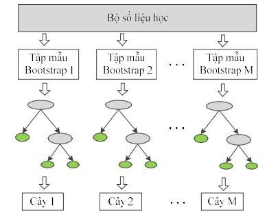
Figure 3.11. The process of building component decision trees
X
Tree 1
Study/test data set
Tree 2
Tree M
y 1
y 2
Study/test results
y M
Result aggregation block (voting method)
- The synthesis of recognition results from M popular decision trees uses crowd voting method to give the final result, as shown in Figure 3.12.
Figure 3.12. Testing process of the RF random forest model
3.3. Neural network coordination to recognize ECG signals using decision tree model
3.3.1. Proposed combination model
Figure 3.13 shows the general diagram of the combined model using multiple single recognition models , where M − number of single recognition models, x in − input ECG signal, P i − are preprocessing and feature extraction blocks, C i − classification blocks, z − final recognition result corresponding to input signal x in .
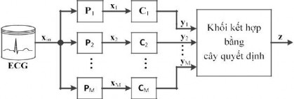
Figure 3.13. General diagram of the combined model using multiple single recognition models
In general, the basic recognition models work independently of the input ECG signal x in which can be from different leads, the preprocessing and feature extraction blocks P i use different methods. As presented in the introduction, the research orientation of the thesis is to use a common preprocessing and feature extraction method P 1 P 2 ... P M for single recognition models C i .
If the problem is to identify K different types of heartbeats, then each single recognition model C i (with i=1, 2,…, M) will have M results y i (with i=1, 2,…, M) represented as vectors (formula 3.1), an ideal vector y i when one value is '1' and all the remaining values are '0', but usually their values often fluctuate in the range [0, 1]. In the thesis, the output results y i from the basic recognition models are combined into a total vector Y (of size M- K) as (3.2) and further processed in the result combination block to draw the final conclusion that the vector z (of size K ) corresponds to the codes of K different types of heartbeats.
- Result of single recognition model C i (with i=1, 2,…, M) :
y i y i1 y i2 ... y iK (3.17)
- Synthetic vector:
Y = [y 1 y 2 ... y M ]
= [y 11 y 12 ...y 1K y 21 y 22 ...y 2K ... y M1 y M2 ...y MK ] (3.18)
Some popular result combination solutions have been proposed by many other studies: Majority voting [11, 16], weighted voting [28, 34], aggregation according to Bayesian conditional probability [28]... In general, these solutions are quite simple, stable, and effective.