Change of Amplitude Amplification Curve When Changing the Resistance Ratio With

Consider the machine shaft model with 3 degrees of freedom (N=3)

The amplitude response of the generalized coordinates is expressed as:

 ˆ e I  t

(4.40)

1 1

2 2

 ˆ e I  t

3 3

 ˆ e I  t

(4.41)

(4.42)

I  t

 a ˆ a e

(4.43)

Substituting N=3, the above dimensionless quantities and equations (4.24), (4.40), (4.41), (4.42) and (4.43) into the system of equations (4.19), we obtain the system of oscillating differential equations:



 ( 2  1)    e I   s t 2 2  2 

 2 ( 

 )  M e I   s t

 

 2 ( 

 2 

 )

sas 1 2

2 seconds

1 2 3

     2 (  2 )

2 3

(4.44)

 2(   2  2 e I  s t)   eI  s t  n  2 

( I 2 2 )

1 assa

 

Solving the system of equations (4.44) we get the complex amplitude of the torsional oscillation of the N = 3rd degree of freedom (third degree of freedom) as:

 ˆ  (  2 2 n 2  2 ) I (  n  2 ) M 

X 3 I  Y 3



s 

(4.45)

in there:



  x (  2 2 n  2  2 )  y

 2 2  n  2 2  2 2 2 n  



3 3   2  2 4  2  2 2n  

(4.46)



3 3 3

Y    x

(  n 2 )  y

 

 3 2 2  n 3 2 n 2 n   ( 4.47)

x  2 2

(4.48)

2 2

y 3  (2  )  1

(4.49)

Compare formulas (4.45), (4.46), (4.47), (4.48) and (4.49) with formulas

(3.20), (3.21), (3.22) and (3.23) we get:

 ˆ 

A 1 I A 2

M 

3  x A y A  I  x A y A k 

(4.50)

3 1 3 3 3 2 3 4 s 

Consider the machine shaft model with 4 degrees of freedom (N=4)

Doing the same with the machine shaft model with 4 degrees of freedom (N=4), we get the system of differential equations for oscillation of the mechanical system:

 ( 2  1)    e I   s t 2 2  2 

 2 ( 

 )  M e I   s t



 

 2 (   2 )

sas 1 2

2

s 1 3 2

  3  s (  4  2  3   2 )

(4.51)



4

   2(  2 )

3 4

 2(   2  2 e I  s t)   eI  s t  n  2 

( I  2 2 )

1 assa

and the complex amplitude of the N = 4th degree of freedom torsional oscillation (fourth degree of freedom) is:

 ˆ 

A 1 I A 2

M 

4  x A y A  I  x A y A k 

(4.52)

4 1 4 3 4 2 4 4 s 

in there:

2 2

x 4  (2  )  1

2 3 2

y 4   2   2(  2)

(4.53)

(4.54)

Comparing the complex amplitude expressions of torsional oscillation of the Nth degree of freedom in machine shaft models with N = 2, 3, 4, … degrees of freedom, we see that these expressions differ only in coefficients x N and y N . From here, the author has the idea of finding a mathematical relationship between the quantities x N , x N-1 , y N and y N-1 to build a general formula of the complex amplitude of torsional oscillation of the Nth degree of freedom in machine shaft models with N degrees of freedom.

- With N = 2 (machine shaft has 2 degrees of freedom)

x 2  1

y 2  2 

(2  1  1)/ 2



k  0

  1  k

(2  1  k )!

 2  1  2 k  ! k !

 2  

2  2  1  2k

- With N = 3 (machine shaft has 3 degrees of freedom)

x  2 2 y

3 2

(3  1)/ 2

2 2

k (3  1  k )!

2 3  1  2k

y 3  (2  )

 1 



k  0

  1 

 3  1  2 k  ! k !

 2  

- With N = 4 (machine shaft has 4 degrees of freedom)

x  (2  2 ) 2  1  y

4 3

y 4   2  

 2( 2

 2) 

(4  1  1)/ 2



k  0

  1  k

(4  1  k )!

 4  1  2 k  ! k !

 2  

2  4  1  2k

- With N = 5 (machine shaft has 5 degrees of freedom)

x  (2  2 ) 3  2( 2  2)  y

5 4

y 5   2  

2  4

 3(2 

2 ) 2

 1 

(5  1)/ 2



k 0

  1 k

(5  1  k )!

 5  1  2 k  ! k !

 2 2

 5  1  2k

…

From the above calculation results we get:

y N    1 

k 0

( N  1  k )!

N  1  2 k  ! k !

 2 2 

N  1  2k

x N y N  1

If N is even: k N = (N-2)/2 ; if N is odd: k N = (N-1)/2

Let y N = A N-1 then x N = A N-2 .

From there we obtain the general formula to determine the complex amplitude of the Nth degree of freedom torsional oscillation in the machine shaft model with N degrees of freedom as follows:

 ˆ 

A 1I A 2

M 

N AA AA  I AA

 AA  k 

(4.55)

N  2 1

N  1 3

N  2 2

N  1 4 s 

Performing complex transformations similar to formulas (3.25) and (3.26) for the case of a single-degree-of-freedom main system (SDOF), we obtain the actual response of the torsional vibration of the Nth degree of freedom as:

A 2 A 2 2  2

ˆ 1 2

N AA  AA  2 2AA  AA  2

(4.56)

N  2 1

N  1 3

N  2 2

N  1 4 

From there we obtain the amplitude-frequency gain function of the Nth degree of freedom in the form:

A 2 A 2 2  2

A A N

1 2

(4.57)

 AA  AA  2 2AA  AA  2

N  2 1

N  1 3

N  2 2

N  1 4 

Where A 1 , A 2 , A 3 , A 4 are coefficients determined from the corresponding single-degree-of-freedom axis model. These coefficients have been determined in formulas (3.20), (3.21), (3.22) and (3.23).

Determine the optimal α ratio

With the amplitude amplification function A determined in formula (4.29), we see that it depends on the 8 dimensionless parameters above including n , μ, η, λ, α, β and the damping ratio ξ. So we can completely determine these parameters so that the amplitude-frequency amplification function reaches its smallest value.

With ξ=0 (no-impedance state) the gain function A in (4.57) has the form:

A 1

A N  2 A 1 A N  1 A 3

A (4.58)

With ξ=∞ (critical barrier state) we have:

A 2

A N  2 A 2 A N  1 A 4

lim A 



(4.59)

Determine fixed points

From the general expression (4.57), determine the amplitude amplification function of the Nth degree of freedom in the machine shaft model with N degrees of freedom. With the machine shaft model with two degrees of freedom (N=2), we have, the amplitude amplification function of the second degree of freedom is:

 (  2 2 n2 2 ) 2  (  n  2 ) 2 2  2

2 2



A 

N  2 

X 2 2 Y 2 

(4.60)

in there:

 2 2  n  2 22 2 2 n  

X   (  2 2 n 2 2 )  (2  2 )   

 2 24 2  2 2n  

   

Y   (  n2)  (2 2)  3 2 2  n3 2 n2 n   

With the machine shaft model with three degrees of freedom (N=3), we have, the amplitude amplification function of the third degree of freedom is:

 (  2 2 n2 2 ) 2  (  n2 ) 2 2  2

3 3



A 

N  3 

X 2 2 Y 2 

(4.61)

in there:



 2 2  n  2 2  2 2 2 n  

X   (2  2 )(  2 2 n 2  2 )  ((2  2 ) 2  1)   

  2  2 4  2  2 2n  

   

Y    (2  2)(  n 2)  ((2  2) 2 1)  3 2 2  n  3 2 n  2 n   

Figures 4.18 and 4.19 respectively describe the change of the amplitude-frequency amplification function of the Nth degree of freedom according to the frequency β for the main system with 2 degrees of freedom (N=2) and the main system with 3 degrees of freedom (N=3) determined from formulas (4.60) and (4.61). From Figures

4.18 and Figure 4.19 we see that all the curves with the value of the viscous damping ratio ξ

all pass through a fixed number of points. The number of these fixed points is 2N. When simulating the amplitude gain function graph of the Nth degree of freedom in the frequency domain with the main system having different number of degrees of freedom and with different values of the damping ratio ξ, the author found that the curves described by (4.60) and (4.61) always pass through fixed points and in the general case, the elevations of these points are different.

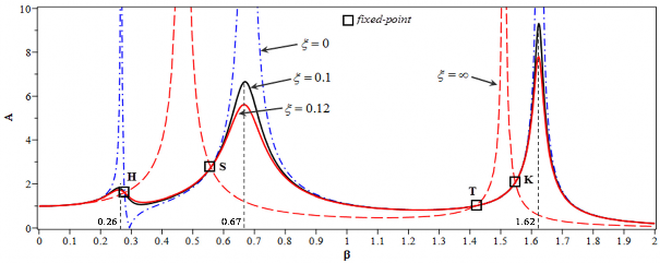
Figure 4.18. Change of amplitude amplification curve when changing the damping ratio with

N = 2, = 0.02, = 1, = 0.5, = 0.8, n = 6 and = 0.2

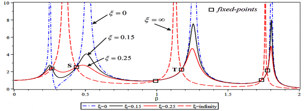
Figure 4.19. Change of amplitude amplification curve when changing the damping ratio with

N = 3, = 0.02, = 1, = 0.5, = 0.8, n = 6 and = 0.2

From figure 4.18 we see that for the main system with N=2 degrees of freedom, there will be 3 resonance peaks (with ξ=0) and 2 resonance peaks (with ξ=∞). For the main system with 3 degrees of freedom, the number of resonance peaks with ξ=0 is 4 peaks and 3 peaks with ξ=∞ (figure 4.19). In general, if the main system has N degrees of freedom, there will be N+1 resonance peaks with the unimpeded state.

(ξ=0) corresponds to N resonance peaks of N degrees of freedom of the main system and 1 additional resonance peak of DVA (subsystem); and in the critical damping state ξ=∞, there will be N resonance peaks. So between these resonance peaks, there are always fixed points.

Similar to the case of the main system with one degree of freedom (section 3.1 of this thesis), the abscissa β j of these fixed points is determined by solving the equation:

 A  0

 

Derivative of the gain function A in (4.57) with respect to the variable ξ we get

 A A  2 A 2 AAA

A 2 A 2 A  2 AA 2 AA

A 2 A 2 A 



N  1 1 2 4

N  2 1 4 N  1 1 2 3

N  2 2 3 N  1

 

N  1 3 4

N  2 1 2

N  1

N  2 1 3 2 4



  1 2 

A 2

A 2 A 2 2 A 2

A 2 A 2 2  2 AA

AA

 AA 2    A 2  A 2 2  2

Conditions for

A 2 A 2 A 2

 A  0 is:

 

 2 A 2 A AAA 

(4.62)

1 4 N  1 1 2 4 N  1 N  2

(4.63)

A 2 A 2 A 2  2 A 2 AA AA

2 3 N  1 2 1 3 N  1 N  2

Add both sides of equation (4.63) with

A 2 A 2 A 2

we have:

A 2 A 2 A 2

A 2 A 2 A 2

 2 A 2 AAAA

1 2 N  2



1 2 N  2 1 4 N  1 1 2 4

N  1 N  2

(4.64)

A 2 A 2 A 2 A 2 A 2 A 2

 2 A 2 AAAA

1 2

From that we have:

A 2

N  2 2 3

AA

N  1 2 1 3

AA  2

N  1

N  2

2

A 2

N  2 2 N  1 4

AA AA  2

(4.65)

1 N  2 1

N  1 3

Equation (4.65) is used to determine the coordinates of fixed points in the general case.

 With the machine shaft model with 2 degrees of freedom (N=2), equation (4.65) becomes:



(  n  2 ) 2

2 2 2 2 2

   n  2 (2 2)( 3  2  2  n 3  2 n   2 n )  

(  n ) 

 2 2  n  2 2 2 2 2 n  

 (  2 2 n  2  2 )  (2  2 )   

  2  2 4  2  2 2n  

   

 With the machine shaft model with 3 degrees of freedom (N=3), equation (4.38) becomes:

(4.66)

(   n  2 ) 2 

(   2 2 n 2  2 ) 2

 (2 2 )(   n  2 )   (2 2 ) 2 1  (  3  2  2  n   3  2 n   2 n )  2



  2 2  n  2 2   2 2 2 n  

 (2  2 )(   2 2 n  2  2 )   (2  2 ) 2  1    

  2  2 4  2   2 2n  

   

(4.67)

Solving equation (4.66) we obtain the values of β j for the machine shaft model with 2 degrees of freedom. Similarly, solving equation (4.67) we obtain the values of β j for the machine shaft model with 3 degrees of freedom.

To determine the optimal parameter α, the values of the amplitude gain function A at two fixed points (corresponding to β 1 and β 2 ) must be equal. There are some values of frequency β, such as β=0.26, β=0.67 and β=1.62, at which resonance occurs (Figure 4.18). The controlled resonance region determined in the optimization design is one of the points closest to β = 1. Therefore, the ratios β 1 and β 2 are chosen so that the controlled β ratio must lie between them. In this way, the two fixed points are chosen as S and T. Solving the equation A S =A T gives the optimal parameter α. Table 4.7 lists the results obtained for the ratio α for N=1, N=2 and N=3.