General Operating Characteristics Curve of a Group of Generators

is expanded. From this, it can be seen that the propeller turbine should not take on much changing load, because with that working mode, the propeller turbine works with low efficiency.

The real gas iso-coefficient curves  of rotary turbines have much larger values

Compared with shaft turbines, the real gas problem in operation for rotary blade turbines is an issue that needs special attention when choosing diameter D 1 as well as when operating.

In the two types of turbines, shaft and propeller, there is an additional 5% power limit line. If the operation exceeds this limit, the turbine efficiency will be greatly reduced. Therefore, when selecting the parameters of this turbine, it is necessary to pay attention to ensure that requirement.

The composite characteristic curve is the model characteristic of a turbine type, it evaluates the working capacity and quality of the model turbine. It is the source document for selecting the working mode of the real turbine.

2. General operating characteristic curve

The general operating characteristic curve is the characteristic curve of a specific turbine with known diameter D 1 and rotation speed n. This characteristic curve is constructed in the coordinate system of water head H and power N, it shows the following curves (Figure 5-7,a):

- Family of iso-efficiency curves  = f (N, H);

- Family of water absorption contour lines Hs = f (N, H);

- The family of lines that limit turbine and generator power.

On the operating characteristic curve we see: point A is the intersection of two limiting curves.

Figure 5-7. Operating characteristic curve.

power of turbine and generator, this point corresponds to water column H tk . We see that when the water column is smaller than the design water column H tk , it cannot generate rated power (showing the power resisted by lack of water column), only when working with water column H  H tk can it generate rated power. General operating characteristic curve

Helps operators determine turbine operating modes, determine parameters at operating modes, and determine turbine power generation capacity.

The operating characteristic curve is also shown in the form of coordinates H ~ Q (Figure 5-7,b).

V. 2. 3. Characteristics of the group of generators

In practice, the TTĐ does not only have one turbine operating but many units (turbine + generator) operating together, so it is necessary to build a general operating characteristic curve for many units. Then the iso-efficiency curves must combine the turbine efficiency curves and generator efficiency curves to get the iso-efficiency curves of a unit. Then build the iso-efficiency curve of the group of units. Below is an example of the operating characteristic curve (  = f(N) of three units (Figure 5-8,a) and the general operating curve of the station with 3 units (Figure 5-8,b).

1. Operating characteristic curve of the group of generators

The operating characteristic curve of a unit shows the relationship between the efficiency and capacity of the unit  1m = f (N) (line I). To draw the relationship curve  2m = f (N) of two identical units, we define the ordinates  and the abscissa N is determined by multiplying the abscissa of one unit by 2 (line II). With 3 identical units, multiply the abscissa of one unit by 3 (line III). With a group of n units, we also draw in the above way.

Figure 5-8,a is the operating characteristic curve of a group of three similar generators:

- When the required load N  N 1 , run one unit;

- When the load requirement is N 1 < N  N 2, it is optimal for units 1 and 2 to work in parallel;

- When the load requirement N > N 2 , all three generators working together is optimal.

Therefore, the operating characteristic curve of the group of generators is the upper envelope 0-1-2-3-4. From

From the characteristic curve of the group of generators, we also realize that to handle the same changing load, if only one generator is installed for the station, although its efficiency  max is higher than the others,

 max each machine receives the load, however the high efficiency working area of a machine is narrow

more, and the working area of many units will be higher. This is very meaningful for stations that take on a lot of changing loads.

2. General operating characteristic curve of the group of generators

The operating characteristic curve of a group of similar units is built on the basis of the operating characteristic curve of a unit by giving a number of water column values H to obtain the corresponding efficiency values  and capacity N of a unit. Multiply those values  , N by 2, 3, 4, ... units. Connect the points with the same efficiency when the generator operates with 1, 2, 3, 4, ... separate units together with smooth curves, we will have the operating characteristic curve of the group of units (Figure 5-8,b).

For stations with different turbines, the overall operating characteristic curve is a set of overall operating characteristic curves of each unit or of groups of similar units operating in different areas.

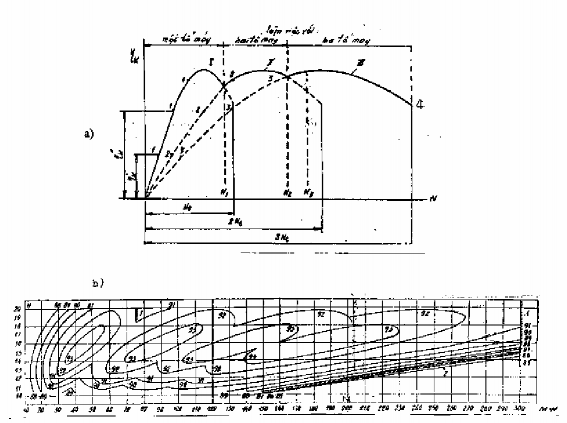
Figure 5-8. Characteristics of the group of generators.

V. 3. CONSTRUCTION OF SYNTHESIS OPERATION CURVE

Part V.2. we have known some characteristic curves of turbines. In which the general characteristic curve is the original curve of a turbine type, it is drawn from model experiments, performed and provided by turbine design and manufacturing agencies. For the field of turbine selection and use, it is necessary to go deeper into the efficiency of energy calculations related to the selected turbine, so we need to know how to build the general operating characteristic curve of a specific turbine. The known data includes:

Working water column from H min to H max , design water column H TK of actual turbine; Rated capacity of turbine and generator;

Standard diameter of real turbine D 1 ;

Synchronous rotation of the nth unit of the real turbine;

The main composite characteristic curve of the model turbine has a D 1M curve .

The following are the contents and steps for calculating and constructing the operating characteristic curve:

1. Constructing iso-efficiency curves = f (N, H)

The diameter of the actual turbine and the model are different, so their efficiency, rotation speed, and flow rate will be different. Therefore, before calculating and drawing the general operating characteristic curve, we must calculate and correct these quantities:

- Correct the real turbine performance according to the model turbine performance:

 T  M (5-3)

When the turbine operating mode changes, the efficiency also changes, it is very difficult to find the efficiency difference  between the two turbines corresponding to each operating mode. Therefore, people rely on the optimal operating mode of the two turbines to calculate  =  T max -  M max and use it for all operating modes. In which  T max ,  M max are determined according to the given formulas (4-24) or (4-25) in chapter IV. If  < 3%, there is no need to adjust the efficiency.

For rotary turbines, adjust the efficiency for the blade angles  , also adjust  according to the optimal working mode of the two turbines.

 max

 M max

- Correct the reference rotation  n' 1 , also based on the optimal working mode to correct

Adjust for all working modes:

n n

(

1 10M

1) and

n n

1 1M

 n ' ; if

If the increment  n' 1  3% then there is no need to correct the reference rotation.

After correction, we create a spreadsheet of the relationship  = f (N, H) for turbine types with some water columns: spreadsheet 5-1, table 5-2 as follows:

Table 5-1. Calculation for turbine Shaft and Propeller.

Correction 

Hmin n ' (n D ): H 1 1 min n ' n '  n ' 1M 1 1 N 9.81 Q ' D 2 H 3/ 2 1 1 min		Htk n ' (n D ): H 1 1 account n ' n '  n ' 1M 1 1 N 9.81  Q ' D 2 H 3/ 2 1 1 account		Hmax n ' (n D ): H 1 1 max n ' n '  n ' 1M 1 1 N 9.81  Q ' D 2 H 3/ 2 1 1 max
 M		Q' 1	N	Q' 1	N	Q' 1	N
1	2	3	4	5	6	7	8

Maybe you are interested!

Column 1: look up on the main composite characteristic curve; Column 2: Take column 1 plus  ;

Column 3, 5, 7: draw horizontal line n' 1M on the main composite characteristic line, meet the points

The corresponding iso-efficiency curve  M will give Q' 1 ;

Columns 4, 6, 8: Calculated according to the formula corresponding to each water column. Table 5-2. Calculated for Rotary Blade turbine.

	Hmin n ' (n D ): H 1 1 min n ' n '  n ' 1M 1 1 N 9.81 Q ' D 2 H 3/ 2 1 1 min				Htk n ' (n D ): H 1 1 account n ' n '  n ' 1M 1 1 N 9.81  Q ' D 2 H 3/ 2 1 1 account				Hmax n ' (n D ): H 1 1 max n ' n '  n ' 1M 1 1 N 9.81  Q ' D 2 H 3/ 2 1 1 max
		 M		Q' 1	N	 M		Q' 1	N	 M		Q' 1	N
1	2	3	4	5	6	7	8	9	10	11	12	13	14

Column 1: Look up on the main composite characteristic curve;

Column 2:  Calculate as presented but take the intersection with the angles  , each angle 

have own adjustment;

Column 3,7,11: draw horizontal line n' 1M on the main composite characteristic line, meet the points

Isogonal lines set  to interpolate sample efficiency; Columns 4, 8, 12: take column  M plus column 2;

Columns 5, 9, 13: corresponding to  M close to find Q' 1 ;

Column 6, 10, 14: Calculate according to the formula above with the corresponding water column

From the calculated data in the above tables (columns 2 ~ 4, 2 ~ 6 and 2 ~ 8 of table 5-1 for shaft and propeller turbines; columns 4 ~ 6, 8 ~ 10, 12 ~ 14 for propeller turbines), draw the working characteristic curves  = f (N), with each water column having one curve (figure 5-9,a).

- Set up the coordinate system H ~ N (figure 5-9,b) with the same abscissa ratio N, placed below the system  ~ N;

+On the H axis of the H ~ N axis system, draw horizontal lines Hmim, H tk, Hmax;

+ On the axis, determine the values of  and draw a horizontal line, intersecting the lines  ~ N. Each water column has two points, for example 1~1' or 2~ 2'; 3~3', drawn down to meet the corresponding water column lines (figure 5-8,b);

+ Connecting points with the same efficiency (with two branches) we get the iso-efficiency curve. With many given values of  we will draw many iso-efficiency curves  = f (N, H)

2. Building capacity-limited roads

The power limit line in the combined operating characteristic curve has two branches formed by the turbine and the generator, they intersect at the design water column ordinate Htk (point A) in figure (5-9,c). The generator power limit line is a vertical line with

abscissa is

N mp

N TB 

 mp

N lm

so lucky

. The turbine power limit curve can be curved.

or approximately straight. The turbine power limit line is constructed as follows:

 Construct the power limit branch for the turbine Shaft and Propeller based on the 5% power limit line on the main general characteristic line of the sample turbine (Figure 5-9,d). Knowing point A ( N mp , H tk ) , it is necessary to determine additional point B ( N B , H min ) and then connect the two points A and B by a straight line.

ok. From

n ' 

n D 1

, draw a horizontal line to meet the constraint line

H min

5% power and find Q ' and interpolate sample efficiency

 M respectively,

Calculate the real turbine efficiency  =

 M +  and determine the turbine power

at point B according to the known formula. With N B , H min can determine point B.



Figure 5-9. Draw the iso-efficiency curves and the power limit curves.

* Construction of the power limiting branch for the Rotary Blade turbine is more complex and has

Two calculation methods. Here is the calculation method proposed by the turbine manufacturer, assuming that: When the water column H > Htk, the turbine capacity is limited by the blade angle  max ;

When the water column H  Htk, the turbine power is limited by the opening a 0max .

We know that the turbine power limiting branch is built from the water column H  Htk, so we calculate to draw the turbine power limiting branch according to the opening a 0 as follows:

- Point A is the intersection of the generator power limit line and Htk which has been easily determined on the coordinate system H ~ N (Figure 5-10,a). Convert the coordinates of point A to coordinates n' 1 ~ Q' 1 on the main general characteristic line of the model turbine (point A') using the following formula:



1tk

n D 1

and



1A 9.81 

N A

D 2 H 3/ 2

therefore Q'

1A'

A 1 tk

H tk

Place point A' (Q' 1A' , n' 1tk ) on figure (9-10,b) and interpolate a 0max .

- Calculate to determine point B corresponding to water column H min and N B , do the following steps:

+ Draw the interpolation contour line a 0max (figure 5-10,b), this line intersects the horizontal line n' 1M corresponding to the water column H min at point B' and interpolate  B ' M and Q' 1 , calculate  B

+ Calculate N B 9.81. 

. Q ' . D 2 . H 3/ 2 . Thus, point B has been determined;

B 1B 1 min

+ Connect point A with B to get the turbine power limiting branch part H  H

Figure 5-10. Construction of auxiliary roads.

3. Construct Hs-suction contour lines

To construct the suction contour H S = f (N, H), we need to draw the auxiliary lines of the water columns on the coordinates N ~ Q 1 ' (figure 5-10,c) based on the calculated results in table 5-1, or table 5-2 above. Then create the calculation table (5-3) below:

- Make table 5-3 with given water columns (at least three water columns H min , H tk , H maxs );

- On the main general characteristic curve (figure 5-10,d) corresponding to each water column, we have n' 1M , draw a horizontal line n' 1M , this line meets the real gas iso-coefficient lines  at the points, at which we interpolate  M , calculate  , and also look up the corresponding Q' 1. With Q' 1, look up the capacity N corresponding to the above water column (figure 5-10,c). Record the above data in columns 1 - 4 and calculate columns 5, 6 and H S = 10 -  /900 - k  H;

- From table 5-3, draw auxiliary lines H S ~ N, each water column has one line (figure 5-10,e);

- Assuming the height values attract HS and drawing horizontal lines meeting the H lines, we get the corresponding N and determine the point with the coordinate pair N, H. With many points, we will draw the lines H S = f (N, H) on the operating characteristic curve.

Table 5-3. Spreadsheet for constructing suction contours

Hmin

n ' (n D ): H

1 1 min

n ' n '  n ' 1M 1 1

k = 1.05 - 1.10

Htk n ' (n D ): H 1 1 account n ' n '  n ' 1M 1 1 k = 1.05 - 1.10	Hmax n ' (n D ): H 1 1 max n ' n '  n ' 1M 1 1 k = 1.05 - 1.10
	Q' 1		N	k  H	HS
1	2	3	4	5	6	...	...

From the results of the calculations as presented above, plotting the same coordinates N ~ H, we can construct the general operating characteristic curve for a specific turbine (Figure 5-7,a).

Comment