Survey on trends in local spending structure movement with economic growth:
Local budget expenditure is divided into development investment expenditure and regular expenditure. The following figure shows the relationship between development investment expenditure and regular expenditure of locality in GDP and economic growth rate.
Figure 3.2 : FDI expenditure/GDP and economic growth rate (%)
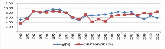
(Source: General Statistics Office & Ministry of Finance, 1990 - 2011)
Local development investment expenditure is considered an expenditure to meet the economic management function of local governments, and at the same time has an important meaning in the current goal of promoting economic growth. From Figure 3.2, we can analyze the preliminary relationship between investment decentralization and growth:
Period 1990 - 1995 : During this period, local investment expenditure in GDP was at an average of 7.16% of GDP, while the economic growth rate increased quite high, at an average of 7.69%. The figure shows the trend of movement in the same direction between the investment expenditure decentralization variable and the growth rate.
Period 1996 - 2000 : After the 1996 Budget Law, along with the impact of the regional financial crisis, economic growth rate
decreased, averaging 5.88%. The rate of decentralized investment spending to localities averaged 7.1% of GDP.
Period 2001 - 2005 : The ratio of decentralized investment expenditure to local governments in GDP averaged 5.47%, economic growth rate during this period reached an average of 7.51%.
Period 2006 - 2011 : After the 2002 State Budget Law, the decentralization of investment spending to local governments tended to increase, at an average of 7.64% of GDP. Due to the impact of the global financial crisis, the average growth rate during this period was only 6.83%.
Thus, in the period 1990-2000, the scale of local investment expenditure moved almost in the direction of GDP growth. This suggests that decentralization of local investment expenditure may be a fundamental factor promoting economic growth in this period. However, in the period 2001-2011, the movement between local investment expenditure and growth rate is not entirely clear. Thus, whether local investment expenditure has an impact on growth or not is still a question that needs to be answered.
Figure 3.3 : DP expenditure/GDP and economic growth rate (%)
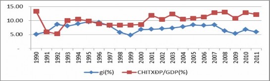
(Source: General Statistics Office & Ministry of Finance, 1990 - 2011)
In the period 1990 - 1995 , local recurrent expenditure in GDP was at an average of 9.14% of GDP; meanwhile, the economic growth rate increased quite high, averaging about 7.69%. In the period 1996 - 2000, it seemed that local recurrent expenditure and growth rate moved in the same direction. Specifically, local recurrent expenditure in GDP tended to decrease at an average of 7.09% of GDP and the average economic growth rate was at 5.88%, lower than the previous period. In the period 2001 - 2011, the relationship between decentralization of local recurrent expenditure compared to GDP and growth rate was unclear. In general, it is necessary to conduct empirical analysis to test this relationship.
3.3.2.3. Revenue decentralization and economic growth
Compared to the 1996 State Budget Law, the 2002 State Budget Law has transferred two revenues, special consumption tax and petroleum fees, from 100% of the central budget revenue to revenues divided between the central budget and local budgets, thereby creating a proactive position associated with increased responsibility for local authorities. Decentralizing revenue sources and expenditure tasks between the central budget and local budgets in the direction of increasing revenue for local budgets and encouraging localities to proactively balance their budgets. Clearly defining and enhancing the proactiveness, associated with the responsibility of ministries, branches, localities, and units in managing the state budget and assets; linking the responsibility of budget management and use with the responsibility of organizing the implementation of political and professional tasks of ministries, branches, localities, units, etc. Those changes not only arouse the proactiveness and promote the resources of localities. That is also the foundation for Vietnam's economic growth.
Figure 3.4 : State budget revenue/GDP and growth rate (%)
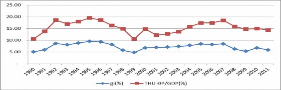
(Source: General Statistics Office & Ministry of Finance, 1990 - 2011)
Figure 3.4 shows that the rate of local budget revenue decentralization in GDP increased rapidly in the period 1990 - 1996, from 5.5% of GDP in 1990 to 9.33% of GDP in 1996. This period witnessed rapid GDP growth from 5.1% in 1990 to 9.33% in 1996. In the period 1997 - 2000, when implementing the State Budget Law 1996, the level of revenue decentralization to local governments was kept stable at over 7.76% of GDP. However, during this period, due to the regional financial crisis, the economic growth rate declined to its lowest level in 1999 at 4.8%. In the period 2001 - 2011, we can see the trend of revenue decentralization and growth moving in the same direction. Local spending needs average 17.69% of GDP, while allocated revenue accounts for 8.68% of GDP (Table 3.2). Thus, allocated revenue only meets about 50% of local spending needs; therefore, localities must receive fiscal transfers from the central government of about 50% to balance the budget.
3.4. Test results and discussion of research results
To test the model using the OLS method, we test the stationarity of the series. If we estimate a model with a time series in which the independent variable is non-stationary, then the OLS assumption is violated. In other words, OLS does not apply to non-stationary series. Another problem related to non-stationarity is that this variable shows an increasing (decreasing) trend and if the dependent variable also has the same trend, when estimating the model, we can obtain a coefficient estimate with high statistical significance and a high R 2. Because the time series can be explained by the behavior in the present, in the past, the degrees
lags and random factors, so in the testing process we test the model lag. After testing the model using the OLS method, we test the model's suitability to assess the reliability of the testing results.
3.4.1. Stationarity test
To test the stationarity of time series variables, test
Traditional Augmented Dickey - Fuller (ADF) with the hypothesis:
H 0 : 0
=> conclusion
Conclusion: has unit root or non-stationary series;
H 1 : 0 => conclusion: zero string
has a unit root or the series is stationary. The important criterion is that if the t-statistic (calculated in the model) for has a negative value greater than the value of the DF table in the Augmented Dickey – Fuller test, then the null hypothesis H 0 is rejected or the variable is stationary or does not have a unit root. The test results are presented in Table 3.3.
Table 3.3 : Results of testing the stationarity of variables in the model
Variable
Delay | t-Statistic | Prob.* | |
gi | 1 | (-2.2632172)*** | 0.0766 |
SI | 0 | (-3.400771)** | 0.0243 |
PGR | 0 | (-7.015842)* | 0.0000 |
dCG | 0 | (-6.135499)* | 0.0001 |
dLG | 0 | (-5.660301)* | 0.0002 |
LG C | 0 | (-2.941203)*** | 0.0574 |
LG I | 0 | (-2.908097)*** | 0.0612 |
LR | 4 | (-3.676897)** | 0.0151 |
TR | 0 | (-2.869733)*** | 0.0659 |
dTOP | 0 | (-5.919251)* | 0.0001 |
inf | 0 | (-3.798081)* | 0.0098 |
Maybe you are interested!
-

 Identify Rating Levels and Rating Scales
zt2i3t4l5ee
zt2a3gstourism,quan lan,quang ninh,ecology,ecotourism,minh chau,van don,geography,geographical basis,tourism development,science
zt2a3ge
zc2o3n4t5e6n7ts
of the islanders. Therefore, this indicator will be divided into two sub-indicators:
a1. Natural tourism attractiveness a2. Cultural tourism attractiveness
b. Tourist capacity
The two island communes in Quan Lan have different capacities to receive tourists. Minh Chau Commune is home to many standard hotels and resorts, attracting high-income domestic and international tourists. Meanwhile, Quan Lan Commune has many motels mainly built and operated by local people, so the scale and quality are not high, and will be suitable for ordinary tourists such as students.
c. Time of exploitation of Quan Lan Island Commune:
Quan Lan tourism is seasonal due to weather and climate conditions and festivals only take place on certain days of the year, specifically in spring. In Quan Lan commune, the period from April to June and from September to November is considered the best time to visit Quan Lan because the cultural tourism activities are mainly associated with festivals taking place during this time.
Minh Chau island commune:
Tourism exploitation time is all year round, because this is a place with a number of tourist attractions with diverse ecosystems such as Bai Tu Long National Park Research Center, Tram forest, Turtle Laying Beach, so besides coming to the beach for tourism and vacation in the summer, Minh Chau will attract research groups to come for tourism combined with research at other times of the year.
d. Sustainability
The sustainability of ecotourism sites in Quan Lan and Minh Chau communes depends on the sensitivity of the ecosystems to climate changes.
landscape. In general, these tourist destinations have a fairly high level of sustainability, because they are natural ecosystems, planned and protected. However, if a large number of tourists gather at certain times, it can exceed the carrying capacity and affect the sustainability of the environment (polluted beaches, damaged trees, animals moving away from their habitats, etc.), then the sustainability of the above ecosystems (natural ecosystems, human ecosystems) will also be affected and become less sustainable.
e. Location and accessibility
Both island communes have ports to take tourists to visit from Van Don wharf:
- Quan Lan – Van Don traffic route:
Phuc Thinh – Viet Anh high-speed boat and Quang Minh high-speed boat, depart at 8am and 2pm from Van Don to Quan Lan, and at 7am and 1pm from Quan Lan to Van Don. There are also wooden boats departing at 7am and 1pm.
- Van Don - Minh Chau traffic route:
Chung Huong high-speed train, Minh Chau train, morning 7:30 and afternoon 13:30 from Van Don to Minh Chau, morning 6:30 and afternoon 13:00 from Minh Chau to Van Don.
f. Infrastructure
Despite receiving investment attention, the issue of infrastructure and technical facilities for tourism on Quan Lan Island is still an issue that needs to be resolved because it has a direct impact on the implementation of ecotourism activities. The minimum conditions for serving tourists such as accommodation, electricity, water, communication, especially medical services, and security work need to be given top priority. Ecotourism spots in Minh Chau commune are assessed to have better infrastructure and technical facilities for tourism because there are quite complete and synchronous conditions for serving tourists, meeting many needs of domestic and foreign tourists.
3.2.1.4. Determine assessment levels and assessment scales
Corresponding to the levels of each criterion, the index is the score of those levels in the order of 4, 3, 2, 1 decreasing according to the standard of each level: very attractive (4), attractive (3), average (2), less attractive (1).
3.2.1.5. Determining the coefficients of the criteria
For the assessment of DLST in the two communes of Quan Lan and Minh Chau islands, the students added evaluation coefficients to show the importance of the criteria and indicators as follows:
Coefficient 3 with criteria: Attractiveness, Exploitation time. These are the 2 most important criteria for attracting tourists to tourism in general and eco-tourism in particular, so they have the highest coefficient.
Coefficient 2 with criteria: Capacity, Infrastructure, Location and accessibility . Because the assessment area is an island commune of Van Don district, the above criteria are selected by the author with appropriate coefficients at the average level.
Coefficient 1 with criteria: Sustainability. Quan Lan has natural and human-made ecotourism sites, with high biodiversity and little impact from local human factors. Most of the ecotourism sites are still wild, so they are highly sustainable.
3.2.1.6. Results of DLST assessment on Quan Lan island
a. Assessment of the potential for natural tourism development
For Minh Chau commune:
+ Natural tourism attractiveness is determined to be very attractive (4 points) and the most important coefficient (coefficient 3), so the score of the Attractiveness criterion is 4 x 3 = 12.
+ Capacity is determined as average (2 points) and the coefficient is quite important (coefficient 2), then the score of Capacity criterion is 2 x 2 = 4.
+ Exploitation time is long (4 points), the most important coefficient (coefficient 3) so the score of the Exploitation time criterion is 4 x 3 = 12.
+ Sustainability is determined as sustainable (4 points), the important coefficient is the average coefficient (coefficient 1), so the score of the Sustainability criterion is 4 x 1 = 4 points
+ Location and accessibility are determined to be quite favorable (2 points), the coefficient is quite important (coefficient 2), the criterion score is 2 x 2 = 4 points.
+ Infrastructure is assessed as good (3 points), the coefficient is quite important (coefficient 2), then the score of the Infrastructure criterion is 3 x 2 = 6 points.
The total score for evaluating DLST in Minh Chau commune according to 6 evaluation criteria is determined as: 12 + 4 + 12 + 4 + 4 + 6 = 42 points
Similar assessment for Quan Lan commune, we have the following table:
Table 3.3: Assessment of the potential for natural ecotourism development in Quan Lan and Minh Chau communes
Attractiveness of self-tourismof course
Capacity
Mining time
Sustainability
Location and accessibility
Infrastructure
Result
Point
DarkMulti
Point
DarkMulti
Point
DarkMulti
Point
DarkMulti
Point
DarkMulti
Point
DarkMulti
CommuneMinh Chau
12
12
4
8
12
12
4
4
4
8
6
8
42/52
Quan CommuneLan
6
12
6
8
9
12
4
4
4
8
4
8
33/52
b. Assessment of the potential for humanistic tourism development
For Quan Lan commune:
+ The attractiveness of human tourism is determined to be very attractive (4 points) and the most important coefficient (coefficient 3), so the score of the Attractiveness criterion is 4 x 3 = 12.
+ Capacity is determined to be large (3 points) and the coefficient is quite important (coefficient 2), then the score of the Capacity criterion is 3 x 2 = 6.
+ Mining time is average (3 points), the most important coefficient (coefficient 3) so the score of the Mining time criterion is 3 x 3 = 9.
+ Sustainability is determined as sustainable (4 points), the important coefficient is the average coefficient (coefficient 1), so the score of the Sustainability criterion is 4 x 1 = 4 points.
+ Location and accessibility are determined to be quite favorable (2 points), the coefficient is quite important (coefficient 2), the criterion score is 2 x 2 = 4 points.
+ Infrastructure is rated as average (2 points), the coefficient is quite important (coefficient 2), then the score of the Infrastructure criterion is 2 x 2 = 4 points.
The total score for evaluating DLST in Quan Lan commune according to 6 evaluation criteria is determined as: 12 + 6 + 6 + 4 + 4 + 4 = 36 points.
Similar assessment with Minh Chau commune we have the following table:
Table 3.4: Assessment of the potential for developing humanistic eco-tourism in Quan Lan and Minh Chau communes
Attractiveness of human tourismliterature
Capacity
Mining time
Sustainability
Location and accessibility
Infrastructure
Result
Point
DarkMulti
Point
DarkMulti
Point
DarkMulti
Point
DarkMulti
Point
DarkMulti
Point
DarkMulti
Quan CommuneLan
12
12
6
8
9
12
4
4
4
8
4
8
39/52
Minh CommuneChau
6
12
4
8
12
12
4
4
4
8
6
8
36/52
Basically, both Minh Chau and Quan Lan localities have quite favorable conditions for developing ecotourism. However, Quan Lan commune has more advantages to develop ecotourism in a humanistic direction, because this is an area with many famous historical relics such as Quan Lan Communal House, Quan Lan Pagoda, Temple worshiping the hero Tran Khanh Du, ... along with local festivals held annually such as the wind praying ceremony (March 15), Quan Lan festival (June 10-19); due to its location near the port and long exploitation time, the beaches in Quan Lan commune (especially Quan Lan beach) are no longer hygienic and clean to ensure the needs of tourists coming to relax and swim; this is also an area with many beautiful landscapes such as Got Beo wind pass, Ong Phong head, Voi Voi cave, but the ability to access these places is still very limited (dirt hill road, lots of gravel and rocks), especially during rainy and windy times; In addition, other natural resources such as mangrove forests and sea worms have not been really exploited for tourism purposes and ecotourism development. On the contrary, Minh Chau commune has more advantages in developing ecotourism in the direction of natural tourism, this is an area with diverse ecosystems such as at Rua De Beach, Bai Tu Long National Park Conservation Center...; Minh Chau beach is highly appreciated for its natural beauty and cleanliness, ranked in the top ten most beautiful beaches in Vietnam; Minh Chau commune is also home to Tram forest with a large area and a purity of up to 90%, suitable for building bridges through the forest (a very effective type of natural ecotourism currently applied by many countries) for tourists to sightsee, as well as for the purpose of studying and researching.
Figure 3.1: Thenmala Forest Bridge (India) Source: https://www.thenmalaecotourism.com/(August 21, 2019)
3.2.2. Using SWOT matrix to evaluate Quan Lan island tourism
General assessment of current tourism activities of Quan Lan island is shown through the following SWOT matrix:
Table 3.5: SWOT matrix evaluating tourism activities on Quan Lan island
Internal agent
Strengths- There is a lot of potential for tourism development, especially natural ecotourism and humanistic ecotourism.- The unskilled labor force is relatively abundant.- resource environmentunpolluted, still
Weaknesses- Poorly developed infrastructure, especially traffic routes to tourist destinations on the island.- The team of professional staff is still weak.- Tourism products in general
quite wild, originalintact
general and DLST in particularalone is monotonous.
External agents
Opportunity- Tourism is a key industry in the socio-economic development strategy of the province and Van Don economic zone.- Quan Lan was selected as a pilot area for eco-tourism development within the framework of the green growth project between Quang Ninh province and the Japanese organization JICA.- The flow of tourists and especially ecotourism in the world tends toincreasing
Challenge- Weather and climate change abnormally.- Competition in tourism products is increasingly fierce, especially with other localities in the province such as Ha Long, Mong Cai...- Awareness of tourists, especially domestic tourists, about ecotourism and nature conservation is not high.
Through summary analysis using SWOT matrix we see that:
To exploit strengths and take advantage of opportunities, it is necessary to:
- Diversify products and service types (build more tourism routes aimed at specific needs of tourists: experiential tourism immersed in nature, spiritual cultural tourism...)
- Effective exploitation of resources and differentiated products (natural resources and human resources)
div.maincontent .p { color: black; font-family:"Times New Roman", serif; font-style: normal; font-weight: normal; text-decoration: none; font-size: 14pt; margin:0pt; } div.maincontent p { color: black; font-family:"Times New Roman", serif; font-style: normal; font-weight: normal; text-decoration: none; font-size: 14pt; margin:0pt; } div.maincontent .s1 { color: black; font-family:"Times New Roman", serif; font-style: normal; font-weight: normal; text-decoration: none; font-size: 13pt; } div.maincontent .s2 { color: black; font-family:"Times New Roman", serif; font-style: normal; font-weight: normal; text-decoration: none; font-size: 13pt; } div.maincontent .s3 { color: #0D0D0D; font-family:"Times New Roman", serif; font-style: normal; font-weight: bold; text-decoration: none; font-size: 14pt; } div.maincontent .s4 { color: black; font-family:"Times New Roman", serif; font-style: italic; font-weight: normal; text-decoration: none; font-size: 14pt; } div.maincontent .s5 { color: black; font-family:"Times New Roman", serif; font-style: italic; font-weight: bold; text-decoration: none; font-size: 14pt; } div.maincontent .s6 { color: black; font-family:"Times New Roman", serif; font-style: italic; font-weight: normal; text-decoration: none; font-size: 14pt; vertical-align: -3pt; } div.maincontent .s7 { color: black; font-family:"Times New Roman", serif; font-style: italic; font-weight: normal; text-decoration: none; font-size: 14pt; vertical-align: -2pt; } div.maincontent .s8 { color: black; font-family:"Times New Roman", serif; font-style: italic; font-weight: normal; text-decoration: none; font-size: 14pt; vertical-align: -1pt; } div.maincontent .s9 { color: black; font-family:"Times New Roman", serif; font-style: normal; font-weight: normal; text-decoration: none; font-size: 14pt; } div.maincontent .s10 { color: black; font-family:"Times New Roman", serif; font-style: normal; font-weight: bold; text-decoration: none; font-size: 14pt; } div.maincontent .s11 { color: black; font-family:"Times New Roman", serif; font-style: normal; font-weight: normal; text-decoration: none; font-size: 14pt; } div.maincontent .s12 { color: black; font-family:Symbol, serif; font-style: normal; font-weight: normal; text-decoration: none; font-size: 14pt; } div.maincontent .s13 { color: black; font-family:Wingdings; font-style: normal; font-weight: normal; text-decoration: none; font-size: 14pt; } div.maincontent .s14 { color: black; font-family:"Times New Roman", serif; font-style: normal; font-weight: normal; text-decoration: none; font-size: 9pt; vertical-align: 5pt; } div.maincontent .s15 { color: black; font-family:"Times New Roman", serif; font-style: normal; font-weight: normal; text-decoration: none; font-size: 9pt; vertical-align: 5pt; } div.maincontent .s16 { color: black; font-family:Cambria, serif; font-style: italic; font-weight: normal; text-decoration: none; font-size: 14pt; } div.maincontent .s17 { color: #080808; font-family:"Times New Roman", serif; font-style: normal; font-weight: bold; text-decoration: none; font-size: 14pt; } div.maincontent .s18 { color: #080808; font-family:"Times New Roman", serif; font-style: normal; font-weight: normal; text-decoration: none; font-size: 14pt; } div.maincontent .s19 { color: black; font-family:"Times New Roman", serif; font-style: normal; font-weight: normal; text-decoration: none; font-size: 11pt; } div.maincontent .s20 { color: black; font-family:"Times New Roman", serif; font-style: normal; font-weight: normal; text-decoration: none; font-size: 10pt; } div.maincontent .s21 { color: black; font-family:"Times New Roman", serif; font-style: normal; font-weight: bold; text-decoration: none; font-size: 11pt; } div.maincontent .s22 { color: black; font-family:"Times New Roman", serif; font-style: normal; font-weight: normal; text-decoration: none; font-size: 11pt; } div.maincontent .s23 { color: black; font-family:"Times New Roman", serif; font-style: italic; font-weight: normal; text-decoration: none; font-size: 14pt; } div.maincontent .s24 { color: #212121; font-family:"Times New Roman", serif; font-style: normal; font-weight: normal; tex
Identify Rating Levels and Rating Scales
zt2i3t4l5ee
zt2a3gstourism,quan lan,quang ninh,ecology,ecotourism,minh chau,van don,geography,geographical basis,tourism development,science
zt2a3ge
zc2o3n4t5e6n7ts
of the islanders. Therefore, this indicator will be divided into two sub-indicators:
a1. Natural tourism attractiveness a2. Cultural tourism attractiveness
b. Tourist capacity
The two island communes in Quan Lan have different capacities to receive tourists. Minh Chau Commune is home to many standard hotels and resorts, attracting high-income domestic and international tourists. Meanwhile, Quan Lan Commune has many motels mainly built and operated by local people, so the scale and quality are not high, and will be suitable for ordinary tourists such as students.
c. Time of exploitation of Quan Lan Island Commune:
Quan Lan tourism is seasonal due to weather and climate conditions and festivals only take place on certain days of the year, specifically in spring. In Quan Lan commune, the period from April to June and from September to November is considered the best time to visit Quan Lan because the cultural tourism activities are mainly associated with festivals taking place during this time.
Minh Chau island commune:
Tourism exploitation time is all year round, because this is a place with a number of tourist attractions with diverse ecosystems such as Bai Tu Long National Park Research Center, Tram forest, Turtle Laying Beach, so besides coming to the beach for tourism and vacation in the summer, Minh Chau will attract research groups to come for tourism combined with research at other times of the year.
d. Sustainability
The sustainability of ecotourism sites in Quan Lan and Minh Chau communes depends on the sensitivity of the ecosystems to climate changes.
landscape. In general, these tourist destinations have a fairly high level of sustainability, because they are natural ecosystems, planned and protected. However, if a large number of tourists gather at certain times, it can exceed the carrying capacity and affect the sustainability of the environment (polluted beaches, damaged trees, animals moving away from their habitats, etc.), then the sustainability of the above ecosystems (natural ecosystems, human ecosystems) will also be affected and become less sustainable.
e. Location and accessibility
Both island communes have ports to take tourists to visit from Van Don wharf:
- Quan Lan – Van Don traffic route:
Phuc Thinh – Viet Anh high-speed boat and Quang Minh high-speed boat, depart at 8am and 2pm from Van Don to Quan Lan, and at 7am and 1pm from Quan Lan to Van Don. There are also wooden boats departing at 7am and 1pm.
- Van Don - Minh Chau traffic route:
Chung Huong high-speed train, Minh Chau train, morning 7:30 and afternoon 13:30 from Van Don to Minh Chau, morning 6:30 and afternoon 13:00 from Minh Chau to Van Don.
f. Infrastructure
Despite receiving investment attention, the issue of infrastructure and technical facilities for tourism on Quan Lan Island is still an issue that needs to be resolved because it has a direct impact on the implementation of ecotourism activities. The minimum conditions for serving tourists such as accommodation, electricity, water, communication, especially medical services, and security work need to be given top priority. Ecotourism spots in Minh Chau commune are assessed to have better infrastructure and technical facilities for tourism because there are quite complete and synchronous conditions for serving tourists, meeting many needs of domestic and foreign tourists.
3.2.1.4. Determine assessment levels and assessment scales
Corresponding to the levels of each criterion, the index is the score of those levels in the order of 4, 3, 2, 1 decreasing according to the standard of each level: very attractive (4), attractive (3), average (2), less attractive (1).
3.2.1.5. Determining the coefficients of the criteria
For the assessment of DLST in the two communes of Quan Lan and Minh Chau islands, the students added evaluation coefficients to show the importance of the criteria and indicators as follows:
Coefficient 3 with criteria: Attractiveness, Exploitation time. These are the 2 most important criteria for attracting tourists to tourism in general and eco-tourism in particular, so they have the highest coefficient.
Coefficient 2 with criteria: Capacity, Infrastructure, Location and accessibility . Because the assessment area is an island commune of Van Don district, the above criteria are selected by the author with appropriate coefficients at the average level.
Coefficient 1 with criteria: Sustainability. Quan Lan has natural and human-made ecotourism sites, with high biodiversity and little impact from local human factors. Most of the ecotourism sites are still wild, so they are highly sustainable.
3.2.1.6. Results of DLST assessment on Quan Lan island
a. Assessment of the potential for natural tourism development
For Minh Chau commune:
+ Natural tourism attractiveness is determined to be very attractive (4 points) and the most important coefficient (coefficient 3), so the score of the Attractiveness criterion is 4 x 3 = 12.
+ Capacity is determined as average (2 points) and the coefficient is quite important (coefficient 2), then the score of Capacity criterion is 2 x 2 = 4.
+ Exploitation time is long (4 points), the most important coefficient (coefficient 3) so the score of the Exploitation time criterion is 4 x 3 = 12.
+ Sustainability is determined as sustainable (4 points), the important coefficient is the average coefficient (coefficient 1), so the score of the Sustainability criterion is 4 x 1 = 4 points
+ Location and accessibility are determined to be quite favorable (2 points), the coefficient is quite important (coefficient 2), the criterion score is 2 x 2 = 4 points.
+ Infrastructure is assessed as good (3 points), the coefficient is quite important (coefficient 2), then the score of the Infrastructure criterion is 3 x 2 = 6 points.
The total score for evaluating DLST in Minh Chau commune according to 6 evaluation criteria is determined as: 12 + 4 + 12 + 4 + 4 + 6 = 42 points
Similar assessment for Quan Lan commune, we have the following table:
Table 3.3: Assessment of the potential for natural ecotourism development in Quan Lan and Minh Chau communes
Attractiveness of self-tourismof course
Capacity
Mining time
Sustainability
Location and accessibility
Infrastructure
Result
Point
DarkMulti
Point
DarkMulti
Point
DarkMulti
Point
DarkMulti
Point
DarkMulti
Point
DarkMulti
CommuneMinh Chau
12
12
4
8
12
12
4
4
4
8
6
8
42/52
Quan CommuneLan
6
12
6
8
9
12
4
4
4
8
4
8
33/52
b. Assessment of the potential for humanistic tourism development
For Quan Lan commune:
+ The attractiveness of human tourism is determined to be very attractive (4 points) and the most important coefficient (coefficient 3), so the score of the Attractiveness criterion is 4 x 3 = 12.
+ Capacity is determined to be large (3 points) and the coefficient is quite important (coefficient 2), then the score of the Capacity criterion is 3 x 2 = 6.
+ Mining time is average (3 points), the most important coefficient (coefficient 3) so the score of the Mining time criterion is 3 x 3 = 9.
+ Sustainability is determined as sustainable (4 points), the important coefficient is the average coefficient (coefficient 1), so the score of the Sustainability criterion is 4 x 1 = 4 points.
+ Location and accessibility are determined to be quite favorable (2 points), the coefficient is quite important (coefficient 2), the criterion score is 2 x 2 = 4 points.
+ Infrastructure is rated as average (2 points), the coefficient is quite important (coefficient 2), then the score of the Infrastructure criterion is 2 x 2 = 4 points.
The total score for evaluating DLST in Quan Lan commune according to 6 evaluation criteria is determined as: 12 + 6 + 6 + 4 + 4 + 4 = 36 points.
Similar assessment with Minh Chau commune we have the following table:
Table 3.4: Assessment of the potential for developing humanistic eco-tourism in Quan Lan and Minh Chau communes
Attractiveness of human tourismliterature
Capacity
Mining time
Sustainability
Location and accessibility
Infrastructure
Result
Point
DarkMulti
Point
DarkMulti
Point
DarkMulti
Point
DarkMulti
Point
DarkMulti
Point
DarkMulti
Quan CommuneLan
12
12
6
8
9
12
4
4
4
8
4
8
39/52
Minh CommuneChau
6
12
4
8
12
12
4
4
4
8
6
8
36/52
Basically, both Minh Chau and Quan Lan localities have quite favorable conditions for developing ecotourism. However, Quan Lan commune has more advantages to develop ecotourism in a humanistic direction, because this is an area with many famous historical relics such as Quan Lan Communal House, Quan Lan Pagoda, Temple worshiping the hero Tran Khanh Du, ... along with local festivals held annually such as the wind praying ceremony (March 15), Quan Lan festival (June 10-19); due to its location near the port and long exploitation time, the beaches in Quan Lan commune (especially Quan Lan beach) are no longer hygienic and clean to ensure the needs of tourists coming to relax and swim; this is also an area with many beautiful landscapes such as Got Beo wind pass, Ong Phong head, Voi Voi cave, but the ability to access these places is still very limited (dirt hill road, lots of gravel and rocks), especially during rainy and windy times; In addition, other natural resources such as mangrove forests and sea worms have not been really exploited for tourism purposes and ecotourism development. On the contrary, Minh Chau commune has more advantages in developing ecotourism in the direction of natural tourism, this is an area with diverse ecosystems such as at Rua De Beach, Bai Tu Long National Park Conservation Center...; Minh Chau beach is highly appreciated for its natural beauty and cleanliness, ranked in the top ten most beautiful beaches in Vietnam; Minh Chau commune is also home to Tram forest with a large area and a purity of up to 90%, suitable for building bridges through the forest (a very effective type of natural ecotourism currently applied by many countries) for tourists to sightsee, as well as for the purpose of studying and researching.
Figure 3.1: Thenmala Forest Bridge (India) Source: https://www.thenmalaecotourism.com/(August 21, 2019)
3.2.2. Using SWOT matrix to evaluate Quan Lan island tourism
General assessment of current tourism activities of Quan Lan island is shown through the following SWOT matrix:
Table 3.5: SWOT matrix evaluating tourism activities on Quan Lan island
Internal agent
Strengths- There is a lot of potential for tourism development, especially natural ecotourism and humanistic ecotourism.- The unskilled labor force is relatively abundant.- resource environmentunpolluted, still
Weaknesses- Poorly developed infrastructure, especially traffic routes to tourist destinations on the island.- The team of professional staff is still weak.- Tourism products in general
quite wild, originalintact
general and DLST in particularalone is monotonous.
External agents
Opportunity- Tourism is a key industry in the socio-economic development strategy of the province and Van Don economic zone.- Quan Lan was selected as a pilot area for eco-tourism development within the framework of the green growth project between Quang Ninh province and the Japanese organization JICA.- The flow of tourists and especially ecotourism in the world tends toincreasing
Challenge- Weather and climate change abnormally.- Competition in tourism products is increasingly fierce, especially with other localities in the province such as Ha Long, Mong Cai...- Awareness of tourists, especially domestic tourists, about ecotourism and nature conservation is not high.
Through summary analysis using SWOT matrix we see that:
To exploit strengths and take advantage of opportunities, it is necessary to:
- Diversify products and service types (build more tourism routes aimed at specific needs of tourists: experiential tourism immersed in nature, spiritual cultural tourism...)
- Effective exploitation of resources and differentiated products (natural resources and human resources)
div.maincontent .p { color: black; font-family:"Times New Roman", serif; font-style: normal; font-weight: normal; text-decoration: none; font-size: 14pt; margin:0pt; } div.maincontent p { color: black; font-family:"Times New Roman", serif; font-style: normal; font-weight: normal; text-decoration: none; font-size: 14pt; margin:0pt; } div.maincontent .s1 { color: black; font-family:"Times New Roman", serif; font-style: normal; font-weight: normal; text-decoration: none; font-size: 13pt; } div.maincontent .s2 { color: black; font-family:"Times New Roman", serif; font-style: normal; font-weight: normal; text-decoration: none; font-size: 13pt; } div.maincontent .s3 { color: #0D0D0D; font-family:"Times New Roman", serif; font-style: normal; font-weight: bold; text-decoration: none; font-size: 14pt; } div.maincontent .s4 { color: black; font-family:"Times New Roman", serif; font-style: italic; font-weight: normal; text-decoration: none; font-size: 14pt; } div.maincontent .s5 { color: black; font-family:"Times New Roman", serif; font-style: italic; font-weight: bold; text-decoration: none; font-size: 14pt; } div.maincontent .s6 { color: black; font-family:"Times New Roman", serif; font-style: italic; font-weight: normal; text-decoration: none; font-size: 14pt; vertical-align: -3pt; } div.maincontent .s7 { color: black; font-family:"Times New Roman", serif; font-style: italic; font-weight: normal; text-decoration: none; font-size: 14pt; vertical-align: -2pt; } div.maincontent .s8 { color: black; font-family:"Times New Roman", serif; font-style: italic; font-weight: normal; text-decoration: none; font-size: 14pt; vertical-align: -1pt; } div.maincontent .s9 { color: black; font-family:"Times New Roman", serif; font-style: normal; font-weight: normal; text-decoration: none; font-size: 14pt; } div.maincontent .s10 { color: black; font-family:"Times New Roman", serif; font-style: normal; font-weight: bold; text-decoration: none; font-size: 14pt; } div.maincontent .s11 { color: black; font-family:"Times New Roman", serif; font-style: normal; font-weight: normal; text-decoration: none; font-size: 14pt; } div.maincontent .s12 { color: black; font-family:Symbol, serif; font-style: normal; font-weight: normal; text-decoration: none; font-size: 14pt; } div.maincontent .s13 { color: black; font-family:Wingdings; font-style: normal; font-weight: normal; text-decoration: none; font-size: 14pt; } div.maincontent .s14 { color: black; font-family:"Times New Roman", serif; font-style: normal; font-weight: normal; text-decoration: none; font-size: 9pt; vertical-align: 5pt; } div.maincontent .s15 { color: black; font-family:"Times New Roman", serif; font-style: normal; font-weight: normal; text-decoration: none; font-size: 9pt; vertical-align: 5pt; } div.maincontent .s16 { color: black; font-family:Cambria, serif; font-style: italic; font-weight: normal; text-decoration: none; font-size: 14pt; } div.maincontent .s17 { color: #080808; font-family:"Times New Roman", serif; font-style: normal; font-weight: bold; text-decoration: none; font-size: 14pt; } div.maincontent .s18 { color: #080808; font-family:"Times New Roman", serif; font-style: normal; font-weight: normal; text-decoration: none; font-size: 14pt; } div.maincontent .s19 { color: black; font-family:"Times New Roman", serif; font-style: normal; font-weight: normal; text-decoration: none; font-size: 11pt; } div.maincontent .s20 { color: black; font-family:"Times New Roman", serif; font-style: normal; font-weight: normal; text-decoration: none; font-size: 10pt; } div.maincontent .s21 { color: black; font-family:"Times New Roman", serif; font-style: normal; font-weight: bold; text-decoration: none; font-size: 11pt; } div.maincontent .s22 { color: black; font-family:"Times New Roman", serif; font-style: normal; font-weight: normal; text-decoration: none; font-size: 11pt; } div.maincontent .s23 { color: black; font-family:"Times New Roman", serif; font-style: italic; font-weight: normal; text-decoration: none; font-size: 14pt; } div.maincontent .s24 { color: #212121; font-family:"Times New Roman", serif; font-style: normal; font-weight: normal; tex -
 Discussion of Quantitative Research Results on the Impact of Control Variables on Financial Performance
 -
 Discussion of Research Results of the First Model
 -
 Research Results on the Relationship Between Exchange Rate Level and FDI Capital in Vietnam and Discussion
 -
 Research Results on the Effects of Fertilization on Growth and Productivity of Planted Forests
Note : (i) t-statistics in parentheses; (ii) *** significant at 10% level, ** significant at 5% level, and * significant at 1% level.
Table 3.3 shows that the variables gi, LG I , LG C , TR are stationary time series with an acceptable significance level of 10%. The variables SI, LR are stationary at a significance level of 5%. The variables PGR, inf are stationary at a significance level of 1%. The remaining variables are non-stationary, the first-order differences of these series have reasonable stationarity at a significance level of 1%. From here, the study will use the variables gi, Si, PGR, dCG, dLG, LG C , LG I , LR, TR, dTOP to test the models.
3.4.2. Experimental results
3.4.2.1. Model testing results 1
Table 3.4 shows the results of estimation 1, examining the impact of local expenditure variables on economic growth. With R 2 of 0.71 and the Heteroskedasticity, LM and Ramsey Reset tests, the model used is appropriate and satisfies the conditions of the OLS method.
The regression results show that the local expenditure variable ( LG ) has a positive impact on economic growth ( gi ) with a significance level of 10%; the trade openness variable ( dTOP) has a positive correlation (+) with economic growth rate with a statistical significance of 10%; especially the economic growth of the current year is strongly affected by the economic growth of the previous year with a significance level of 1%. However, the model has not detected the impact of the variables CG, SI, PGR and inf on economic growth.
Table 3.4 : Model 1 estimation results
Variable
coefficient | Std. Error | t-Statistic | Prob. | |
C | 1.289088 | 2.415077 | 0.533767 | 0.6025 |
SI | -0.027761 | 0.027618 | -1.005183 | 0.3332 |
PGR | 0.585889 | 0.476116 | 1.230559 | 0.2403 |
dCG | 0.175565 | 0.227827 | 0.770604 | 0.4547 |
dLG | 0.251065 | 0.139507 | 1.799663 | 0.0952 |
dTOP | 0.047593 | 0.026401 | 1.802695 | 0.0947 |
inf | 0.033715 | 0.027504 | 1.225807 | 0.2420 |
gi(-1) | 0.614837 | 0.153629 | 4.002093 | 0.0015 |
R-squared | 0.716653 | Akaike info criterion | 2.891225 | |
Adjusted R-squared | 0.564082 | Schwarz criterion | 3.289139 | |
F-statistic | 4.697171 | Hannan-Quinn critic. | 2.977583 | |
Prob(F-statistic) | 0.007975 | Durbin-Watson statistics | 1.911280 | |
Model suitability testing: | ||||
Heteroskedasticity Test: Breusch-Pagan-Godfrey | ||||
F-statistic | 0.618802 | Prob. F(7,13) | 0.7321 | |
Breusch-Godfrey Serial Correlation LM Test: | ||||
F-statistic | 0.238854 | Prob. F(2,11) | 0.7915 | |
Ramsey RESET Test | ||||
F-Satistic | 0.0983 | Prob. F(1,12) | 0.7593 | |
3.4.2.2. Model 2 testing results
Table 3.5 describes the results of estimating model 2, examining the impact of local investment and recurrent expenditure variables on economic growth. With R 2 of 0.74 and using Heteroskedasticity, LM and Ramsey Reset tests, the results show that the model is suitable and satisfies the conditions of the OLS method.
When adding two more variables, local investment expenditure ( LG I ) and local recurrent expenditure ( LG C ), to the model, the results show that the variable LG I has a positive impact on growth with a significance level of 10%; while the variable LG C's impact on economic growth is not statistically significant.
Table 3.5 : Model 2 estimation results
Variable
coefficient | Std. Error | t-Statistic | Prob. | |
C | -0.576459 | 2.702478 | -0.213308 | 0.8347 |
SI | -0.032552 | 0.042686 | -0.762580 | 0.4604 |
PGR | 0.425655 | 0.491807 | 0.865493 | 0.4037 |
dCG | 0.445368 | 0.242120 | 1.839455 | 0.0907 |
LG I | 0.345461 | 0.173871 | 1.986877 | 0.0703 |
LG C | 0.094115 | 0.175411 | 0.536543 | 0.6014 |
dTOP | 0.079051 | 0.026806 | 2.949021 | 0.0122 |
Inf | 0.028722 | 0.026348 | 1.090104 | 0.2971 |
gi(-1) | 0.475078 | 0.168263 | 2.823421 | 0.0154 |
R-squared | 0.740721 | Akaike info criterion | 2.897697 | |
Adjusted R-squared | 0.567868 | Schwarz criterion | 3.345350 | |
F-statistic | 4.285272 | Hannan-Quinn critic. | 2.994850 | |
Prob(F-statistic) | 0.012069 | Durbin-Watson statistics | 1.505323 | |
Model suitability testing: | ||||
Heteroskedasticity Test: Breusch-Pagan-Godfrey | ||||
F-statistic | 0.178742 | Prob. F(8,12) | 0.9896 | |
Breusch-Godfrey Serial Correlation LM Test: | ||||
F-statistic | 1.098084 | Prob. F(2,10) | 0.3706 | |
Ramsey RESET Test | ||||
F.statistic | 0.202110 | Prob.F(1,11) | 0.6618 | |