school (Chi-square = 2863.435; df = 1414; Chi-square /df = 2.025; GFI = 0.856; TLI
= 0.910; CFI = 0.914; RMSEA = 0.039), demonstrating that the competitive model is suitable for
market data
Table 4.12: Results of testing the causal relationship between concepts in
competitive model (standardization)
Relationship
Estimate medium | Standard Deviation (SE) | Value to Deadline (CR) | level of intention meaning (P) | |
RAOCAN ---> DONGCO | -0.622 | 0.028 | -8,238 | *** |
RAOCAN ---> HADDEN | -0.169 | 0.037 | -2,306 | 0.021 |
RAOCAN ---> LUACHON | -0.112 | 0.030 | -2,306 | 0.021 |
DONGCO ---> HADDEN | 0.774 | 0.177 | 6,105 | *** |
DONGCO ---> LUACHING | 0.440 | 0.298 | 2,534 | 0.011 |
DONGCO ---> THUGIAN | 0.491 | |||
ENGINEERING ---> KNOWLEDGE | 0.302 | 0.117 | 5,529 | *** |
DONGCO ---> QUANHE | 0.428 | 0.219 | 7,001 | *** |
DONGCO ---> PRESTIGE | 0.737 | 0.214 | 8,849 | *** |
HADDEN ---> LUACHON | 0.402 | 0.196 | 2,525 | 0.012 |
HADDEN ---> TUNHIEN | 0.599 | |||
HADDEN ---> VANHOA | 0.524 | 0.076 | 8,479 | *** |
HADDEN ---> MTRUONG | 0.667 | 0.102 | 9,392 | *** |
HADDEN ---> HTCHUNG | 0.763 | 0.112 | 9,759 | *** |
HADDEN ---> HTDLICH | 0.698 | 0.112 | 10,703 | *** |
HADDEN ---> BKKHI | 0.704 | 0.111 | 10,025 | *** |
Maybe you are interested!
-

 Results of Testing Cronbach's Alpha Coefficient of Independent Variable
 -
 The relationship between travel motivation, destination image and destination choice - A case study of Binh Dinh province tourism destination - 1
 -
 Business Results of Quang Binh Tourism Industry in the Period 2014 - 2019
 -
 Practical Research Results on Event Organization Skills of Tourism Students
 -
 Testing the Differences in Student Satisfaction with the Quality of Training Services at the Faculty of Tourism, University of Industry

***: p < 0.001
Source: Results of processing from author's survey data
The SEM analysis results of both the theoretical model and the competitive model are consistent with the market data and the hypotheses are accepted at the 5% significance level. However, compared to the theoretical research model, the competitive model has a difference when comparing the Chi-square value and the number of degrees of freedom. Indeed, if comparing the Chi-square value, the difference between the two models is 141.321 (3004.756
– 2863.435) with 1 (1415 – 1414) degrees of freedom. The results of the competing model show that there are more possible relationships supported by theory. At the same time, according to the estimation results, the Squared Multiple Correlations index of destination choice is 0.799, meaning that the above concepts explain 79.9%
variation of destination choice. More importantly, the hypothesis built in the competitive model ( H 7: There is a negative relationship between tourists' travel barriers and travel motivation) is statistically significant with p = 0.000 (Table 4.12), so we decided to accept this hypothesis. This is a new finding of this study because the relationship between travel barriers and travel motivation has not been tested in previous studies in the tourism sector.
Thus, the competitive model improves the model's fit to the data and a new relationship is added in the competitive model that has been accepted. Therefore, compared with the theoretical research model, the competitive model is more suitable and comprehensive to explain the market reality. Therefore, in this study, the author uses the competitive model instead of the original theoretical model. On the other hand, in the process of estimating the measurement models and the structural models (theoretical and competitive models), one or more error variances with negative values do not appear, so the Heywood phenomenon does not appear in any model.
4.4.3. Testing research hypotheses
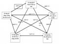
As presented in Sections 4.2 and 4.3, the results of the evaluation of the scales through Cronbach's alpha, EFA and CFA, the initial research hypotheses have not changed. The results of testing the competitive model (instead of the original official theoretical model) have no concepts eliminated and all relationships are statistically significant at the 95% confidence level, so we keep the competitive model (Figure 4.6) with 7 research hypotheses: H 1 , H 2 , H 3 , H 4 , H 5 , H 6 , H 7 .
Estimated results (Table 4.12), excluding the impact of the barrier factor, are
If the number has a negative sign, the weights of the remaining factors are all positive (+) and all are statistically significant (p≤ 0.05), showing that tourism barriers (RAOCAN) have a negative impact on tourism motivation (DONGCO), destination image (HADDEN) and destination choice (LUACHON); conversely, the concepts of tourism motivation (DONGCO) have a positive impact on destination image (HADDEN) as well as destination choice (LUACHON); and finally destination image (HADDEN) has a positive impact on destination choice (LUACHON). This proves that:
H 1 : There is a positive relationship between travel motivation and destination image : accepted.
H 2 : There is a positive relationship between travel motivation and destination choice : accepted.
H 3 . There is a positive relationship between destination image and destination choice : accepted.
H 4 : There is a negative relationship between tourism barriers and destination image : acceptance.
H 5 : There is a negative relationship between travel barriers and destination choice : accepted.
H 7 : There is a negative relationship between travel barriers and travel motivations :
accepted
Hypothesis H 6 will be tested in Section 4.5 next.
4.5. Multi-group structure analysis
4.5.1. Testing for differences according to sociodemographic characteristics of tourists
4.5.1.1. Testing for differences by nationality
According to the nationality of tourists, tourist data is divided into two groups: (1) domestic tourists and (2) international tourists.
SEM results of the variable model for two groups of tourists by nationality: Chi-square = 4,505.393; df = 2828; p = 0.000; Chi-square/df = 1.593; GFI = 0.802; TLI = 0.898; CFI = 0.903; RMSEA = 0.030 (Appendix 8.1a).
SEM results of invariant model for two groups of tourists by nationality: Chi-square = 4,524.464; df = 2834; p = 0.000; Chi-square/df = 1.596; GFI = 0.801; TLI = 0.897; CFI = 0.902; RMSEA = 0.030 (Appendix 8.1b).
Demonstrate both variable and partial invariant models of two customer groups
Travel by nationality is consistent with market data.
The results of testing the difference in compatibility indicators between the variable model and the partial invariant model (Table 4.13) show that the difference between the two models is statistically significant (p = 0.004 < 0.05). Therefore, the variable model is selected and allowed.
concluded that differences in tourists' nationalities have different impacts on the relationship
Relationship between travel motivation, destination image and tourist destination choice.
Table 4.13: Differences between compatibility indicators by nationality
Comparison model
χ 2 | df | p | NFI | RFI | IFI | TLI | CFI | |
Variable model | 4505,393 | 2828 | 0 | 0.777 | 0.766 | 0.904 | 0.898 | 0.903 |
Partial invariant model | 4524,464 | 2834 | 0 | 0.777 | 0.766 | 0.903 | 0.897 | 0.902 |
Differentiation value | 8,439 | 6 | 0.004 | -0.000 | -0.000 | -0.001 | -0.001 | -0.001 |
Source: Results of processing from author's survey data
Table 4.14: Estimated relationships between concepts in the nationality-variable model (standardized)
Relationship
Domestic tourists | International tourists | |||||||
λ | SE | CR | P | λ | SE | CR | P | |
RAOCAN ---> DONGCO | -0.577 | 0.029 | -6,345 | *** | -0.709 | 0.061 | -5,368 | *** |
RAOCAN ---> HADDEN | -0.291 | 0.034 | -3,758 | *** | 0.154 | 0.146 | ,695 | ,487 |
RAOCAN ---> LUACHON | -0.125 | 0.038 | -2,069 | 0.039 | -0.298 | 0.174 | -1,096 | 0.273 |
DONGCO ---> HADDEN | 0.680 | 0.186 | 4,983 | *** | 1,045 | 0.464 | 3,213 | ,001 |
DONGCO ---> LUACHING | 0.542 | 0.352 | 3,018 | 0.003 | -0.477 | 1,510 | -0.436 | 0.663 |
DONGCO ---> THUGIAN | 0.487 | 0.508 | ||||||
ENGINEERING ---> KNOWLEDGE | 0.290 | 0.155 | 4,312 | *** | 0.319 | 0.174 | 3,519 | *** |
DONGCO ---> QUANHE | 0.460 | 0.338 | 5,850 | *** | 0.323 | 0.230 | 3,503 | *** |
DONGCO ---> PRESTIGE | 0.781 | 0.314 | 7,045 | *** | 0.667 | 0.263 | 5,490 | *** |
HADDEN ---> LUACHON | 0.327 | 0.247 | 1,908 | 0.056 | 1,120 | 0.882 | 1,229 | 0.219 |
HADDEN ---> TUNHIEN | 0.555 | 0.673 | ||||||
HADDEN ---> VANHOA | 0.453 | 0.083 | 5,582 | *** | 0.660 | 0.140 | 6,733 | *** |
HADDEN ---> MTRUONG | 0.645 | 0.154 | 7,372 | *** | 0.704 | 0.129 | 5,538 | *** |
HADDEN ---> HTCHUNG | 0.762 | 0.162 | 7,372 | *** | 0.746 | 0.149 | 6,377 | *** |
HADDEN ---> HTDLICH | 0.736 | 0.179 | 8,406 | *** | 0.635 | 0.127 | 6,302 | *** |
HADDEN ---> BKKHI | 0.704 | 0.155 | 7,478 | *** | 0.707 | 0.155 | 6,732 | *** |
Source: Results of processing from author's survey data
The results of estimating the relationship between the concepts in the variable model (Table 4.14) show that the main differences between tourists of different nationalities are:
While travel motivation, destination image and travel barriers play an important role (λ = 0.542; 0.3278 and -0.125 respectively) in determining destination choice for domestic tourists at a significance level of 5% (10% for destination image), for international tourists these factors are not statistically significant (p = 0.663; 0.219; 0.273 respectively, all greater than 0.05). This conclusion means that if there are the same factors determining destination choice according to the nationality of tourists, there are differences in the impact (importance) of these factors between groups of tourists with different nationalities.
4.5.1.2. Testing for gender differences
According to the gender of tourists, the tourist data is divided into two groups: (1) male tourists and (2) female tourists.
SEM results of the variable model for two groups of tourists by gender: Chi-square = 4553.183; df = 2828; p = 0.000; Chi-square/df = 1.610; GFI = 0.799; TLI = 0.895; CFI = 0.900; RMSEA = 0.030 (Appendix 8.2a).
SEM results of invariant model for two groups of tourists by gender: Chi-square = 4558.939; df = 2834; p = 0.000; Chi-square/df = 1.609; GFI = 0.798; TLI = 0.895; CFI = 0.900; RMSEA = 0.030 (Appendix 8.2b).
Demonstrate both variable and partial invariant models of two customer groups
Gendered travel is consistent with market data.
Table 4.15: Differences between compatibility indicators by gender
Comparison model
χ 2 | df | p | NFI | RFI | IFI | TLI | CFI | |
Variable model | 4553,183 | 2828 | 0 | 0.774 | 0.763 | 0.901 | 0.895 | 0.9 |
Partial invariant model | 4558,939 | 2834 | 0 | 0.774 | 0.763 | 0.901 | 0.895 | 0.9 |
Differentiation value | 5,756 | 6 | 0.451 | -0.000 | -0.000 | 0.000 | 0.000 | 0.000 |
Source: Results of processing from author's survey data
The results of testing the difference in compatibility indicators between the variable model and the partial invariant model (Table 4.15) show that the difference between the two models is not statistically significant (p = 0.451 > 0.05). Therefore, the invariant model is selected and allows to conclude that the difference in gender of tourists has no different impact.
relationship between travel motivation, destination image and destination choice
tourism.
4.5.1.3. Testing for age differences
According to the age of tourists, the data on interviewed tourists were divided into three age groups: from 18 to 35, from 36 to 55 and over 55. Of which, the number of tourists focused mainly on the group of tourists aged from 18 to 35 (416 tourists, accounting for 62%); followed by the group of tourists aged from 36 to 55 (197 tourists, accounting for 29.36%); the rest was the group of tourists aged over 56 (58 tourists, accounting for 8.64%). Therefore, to increase the reliability of the test, the author grouped them into two groups: (1) from 18 to 35 and (2) 36 years old and over.
SEM results of the variable model for two groups of tourists by age: Chi-square = 4534.341; df = 2828; p = 0.000; Chi-square/df = 1.603; GFI = 0.801; TLI = 0.896; CFI = 0.901; RMSEA = 0.030 (Appendix 8.3a).
SEM results of invariant model for two groups of tourists by age: Chi-square = 4539.449; df = 2834; p = 0.000; Chi-square/df = 1.602; GFI = 0.800; TLI = 0.896; CFI = 0.901; RMSEA = 0.030 (Appendix 8.3b).
Demonstrate both variable and partial invariant models of two customer groups
Travel by age is consistent with market data.
Table 4.16: Differences between compatibility indicators by age
Comparison model
χ 2 | df | p | NFI | RFI | IFI | TLI | CFI | |
Variable model | 4534,341 | 2828 | 0 | 0.775 | 0.764 | 0.902 | 0.896 | 0.901 |
Partial invariant model | 4539,449 | 2833 | 0 | 0.775 | 0.764 | 0.902 | 0.896 | 0.901 |
Differentiation value | 5,108 | 6 | 0.530 | 0.000 | 0.000 | 0.000 | 0.000 | 0.000 |
Source: Results of processing from author's survey data
The results of testing the difference in compatibility indicators between the variable model and the partial invariant model (Table 4.16) show that the difference between the two models is not statistically significant (p = 0.530 > 0.05). Therefore, the invariant model is selected and allows to conclude that the difference in age of tourists does not have a different impact on the relationship between travel motivation, destination image and travel destination choice.
4.5.1.4. Testing for differences by educational level
According to the educational level of tourists, the data on interviewed tourists were divided into four groups: secondary school; secondary school, college; university; post-graduate. In which, the number of tourists focused mainly on the group of tourists with university education (332 tourists, accounting for 49.48%); followed by the group of tourists with secondary school, college education (159 tourists, accounting for 23.69%) and the group of tourists with secondary education (93 tourists, accounting for 13.86%); the rest was the group of tourists with post-graduate education (87 tourists, accounting for 12.97%). Therefore, to increase the reliability of the test, the author grouped them into two groups: (1) not having attended university and (2) having attended university.
SEM results of the variable model for two groups of tourists according to education level: Chi-square = 4602.721; df = 2828; p = 0.000; Chi-square/df = 1.628; GFI = 0.799; TLI = 0.892; CFI = 0.897; RMSEA = 0.031 (Appendix 8.4a).
SEM results of invariant model for two tourist groups according to education level: Chi-square = 4611.151; df = 2834; p = 0.000; Chi-square/df = 1.627; GFI = 0.799; TLI = 0.892; CFI = 0.897; RMSEA = 0.031 (Appendix 8.4b).
Demonstrate both variable and partial invariant models of two customer groups
Travel by education level is consistent with market data.
Table 4.17: Differences between compatibility indicators by educational level
Comparison model
χ 2 | df | p | NFI | RFI | IFI | TLI | CFI | |
Variable model | 4602,721 | 2828 | 0 | 0.773 | 0.761 | 0.898 | 0.892 | 0.897 |
Partial invariant model | 4611,151 | 2834 | 0 | 0.772 | 0.761 | 0.898 | 0.892 | 0.897 |
Differentiation value | 8,430 | 6 | 0.208 | -0.001 | 0.000 | 0.000 | 0.000 | 0.000 |
Source: Results of processing from author's survey data
The results of testing the difference in compatibility indicators between the variable model and the partial invariant model (Table 4.17) show that the difference between the two models is not statistically significant (p = 0.208 > 0.05). Therefore, the invariant model was selected and allows to conclude that the difference in tourists' education level does not have a different impact on the relationship between travel motivation, destination image and travel destination choice.
4.5.1.5. Testing for occupational differences
According to the occupation of tourists, the data on interviewed tourists were divided into four groups: businessmen; state employees; workers; other groups. Of which, the number of tourists focused mainly on the group of tourists with other occupations (309 tourists, accounting for 46.05%); followed by the group of tourists who were state employees (195 tourists, accounting for 29.06%) and the group of tourists who were workers (89 tourists, accounting for 13.26%); the rest were the group of tourists who were businessmen (78 tourists, accounting for 11.63%). Initially when testing SEM with 4 individual groups, the results of the values did not meet the requirements (Chi-square = 8818.657; df = 5656; p = 0.000; Chi-square/df = 1.559; GFI = 0.705; TLI = 0.822;
CFI = 0.831; RMSEA = 0.029). Therefore, to increase the reliability of the test, the author grouped the participants into two groups: (1) State employees and workers and (2) Businessmen and other groups.
SEM results of the variable model for two groups of tourists by occupation: Chi-square = 4643.974; df = 2828; p = 0.000; Chi-square/df = 1.642; GFI = 0.796; TLI = 0.890; CFI = 0.895; RMSEA = 0.031 (Appendix 8.5a).
SEM results of invariant model for two groups of tourists by occupation: Chi-square = 4652.625; df = 2834; p = 0.000; Chi-square/df = 1.642; GFI = 0.796; TLI = 0.890; CFI = 0.895; RMSEA = 0.031 (Appendix 8.5b).
Demonstrate both variable and partial invariant models of two customer groups
Career travel is consistent with market data.
Table 4.18: Differences between compatibility indicators by occupation
Comparison model
χ 2 | df | p | NFI | RFI | IFI | TLI | CFI | |
Variable model | 4643,974 | 2828 | 0 | 0.771 | 0.76 | 0.896 | 0.89 | 0.895 |
Partial invariant model | 4652,625 | 2834 | 0 | 0.771 | 0.76 | 0.896 | 0.89 | 0.895 |
Differentiation value | 8,651 | 6 | 0.194 | 0.000 | 0.000 | 0.000 | 0.000 | 0.000 |
Source: Results of processing from author's survey data
The results of testing the difference in compatibility indicators between the variable model and the partial invariant model (Table 4.18) show that the difference between the two models is not statistically significant (p = 0.194 > 0.05). Therefore, the invariant model was selected and