Image How to Identify a True Disc Herniation [45].

. Nerve root compression: assessed by the number of compressed nerve roots, specifically one root, two roots or more [43], [41].

. Disc bulge: widening of the disc around but still following the joint border (50 – 100% of the disc circumference, but < 3mm) (Figure 2.4) [45].

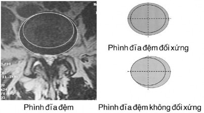
Figure 2.4. Image of how to identify disc bulge [45].

. Disc protrusion: when the height of the herniated mass is smaller than the base of the herniated disc (Figure

2.5) [45].

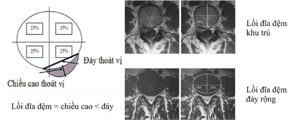
Figure 2.5. Image of how to identify disc protrusion [45].

True hernia: when the height of the hernia mass is larger than the hernia base (Figure 2.6) [45].

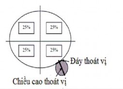
Figure 2.6. Image of how to identify a true disc herniation [45].

+ Sagittal T1W and T2W images of the lateral cross-section reveal narrowing of the graft hole:

evaluated by comparison with adjacent upper and lower graft holes above [46].

+ Measure the size of the lumbar spinal canal at the location of disc herniation: anterior-posterior diameter of the spinal canal on the T2-weighted sagittal image at the location of herniation, anterior-posterior diameter

– behind the spinal canal on T2 cross-sectional image at the site of herniation.

. Assess spinal canal stenosis through the size of the anterior-posterior diameter on longitudinal and transverse images, compared with the size of the spinal canal according to the authors Tran Trung, Moeller, Modic MT in Table 2.4, Figure 2.7. [38], [46].

Table 2.2. Criteria for classifying the degree of lumbar spinal stenosis on magnetic resonance imaging (Moeller 2007).

Front - rear diameter

of the spinal canal

Spinal stenosis
Light	Fit	Heavy	Very heavy

Maybe you are interested!

Size (mm) 10 – 12 7 – 9 4 – 6 0 – 3

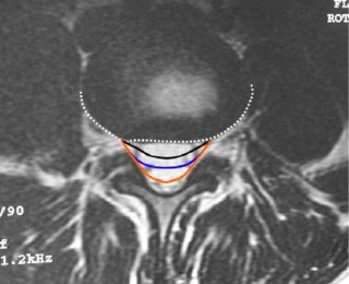
Figure 2.7. Image of how to determine spinal stenosis [45].

- Parameters collected when examining magnetic resonance imaging include:

+ Location of herniated disc.

+ Disc herniation (central posterior, right posterior, left posterior, into the graft foramen).

+ Location of bulging disc.

+ Location of torn disc annulus.

+ Actual location of disc herniation.

+ Herniated disc location with loose fragments.

+ Location of nerve root compression.

+ Assess the degree of spinal stenosis.

+ Other associated injuries: reduced physiological curve, reduced vertebral body height, osteophytes, slipped vertebral body, hypertrophy of ligamentum flavum, hypertrophy of posterior longitudinal ligament, synovial cyst of lateral joint mass, destruction of vertebral isthmus, lumbar scoliosis, radiculitis, etc. (Appendix 2).

Thus, after performing a lumbar spine MRI test, a definitive imaging diagnosis of lumbar spine disc herniation at a specific location will be made.

2.2.4.3. Patients undergo electrodiagnostic testing.

The patient was tested at the Neurology Department - Viet Tiep Friendship Hospital using the Neuropack machine of Nihon - Konden Japan, placed in an air-conditioned room (average temperature from 24 - 26 0 C). The test was performed directly by the researcher, using the following techniques:

* Nerve conduction study:

- Measurement of conduction of deep peroneal nerve:

+ Preparation: patient lies on back, legs stretched.

+ Technique:

. Electrode placement: recording electrode at the extensor digitorum brevis muscle in the dorsum of the foot (muscle belly). Reference electrode placed at the base of the little toe (metatarsal joint of the little toe). Ground electrode placed at the dorsum of the foot, between the 2 electrodes: recording electrode and stimulating electrode.

. Stimulation of the deep peroneal nerve at 3 locations: (1) at the ankle just above the anterior junction of the medial and lateral malleolus. (2) below the fibular head (2 cm) and (3) above the fibular head (lateral to the popliteal fossa, 9 cm from stimulation point (2), on the course of the deep peroneal nerve:

Figure 2.8. Schematic diagram of electrode connection for recording motor conduction of the deep peroneal nerve [34].

- Measurement of tibial nerve conduction :

+ Preparation: patient lies on side, legs stretched.

+ Technique: . Electrode placement: recording electrode at the abductor hallucis longus muscle (muscle belly, scaphoid process 1 cm down and 1 cm back). Electrode

The reference electrode is placed at the base of the big toe (metatarsal joint of the thumb). The ground electrode is placed at the instep of the foot, between the two electrodes: the recording electrode and the stimulating electrode.

. Stimulation at: stimulation point (1) is placed at the posterior border of the medial malleolus on the course of the posterior tibial nerve, 9 cm from the recording electrode. Stimulation point

(2) at the popliteal fossa on the course of the posterior tibial nerve:

Figure 2.9. Schematic diagram of electrode connection for recording motor conduction of the tibial nerve [34].

- Calf nerve conduction measurement:

+ Preparation: patient lies prone, legs stretched.

+ Technique (we use reverse recording method):

. Electrode placement: recording electrode at the back of the ankle (behind the outer malleolus). Reference electrode placed 3 cm below the recording electrode. Ground electrode placed above the ankle, between the 2 electrodes: recording electrode and stimulating electrode.

Stimulation: posterior, lateral calf stimulation point on the course of the calf nerve, 14 cm from the recording electrode:

Figure 2.10. Schematic diagram of electrode connection for recording sensory conduction of the calf nerve [34].

- Measurement of conduction of the superficial peroneal nerve:

+ Preparation: patient lies on back, legs stretched.

+ Technique (we use reverse recording method):

. Electrode placement: recording electrode at the outer part of the ankle (tibialis anterior tendon and lateral malleolus). Reference electrode placed 3 cm below the recording electrode. Ground electrode placed at the instep, between the 2 electrodes: recording electrode and stimulating electrode.

Stimulation: stimulation point on the lateral aspect of the calf on the course of the superficial peroneal nerve, 14 cm from the recording electrode:

Figure 2.11. Schematic diagram of electrode connection for recording sensory conduction of the superficial peroneal nerve [34].

- F wave recording: the method of recording F waves of the deep peroneal nerve and the tibial nerve is similar to the method of recording motor conduction of these two nerves, the only difference is: when stimulating, we rotate the negative electrode toward the base of the limb.

+ Technique: electrical stimulation pulses have a duration of about 0.5 - 1ms, frequency 0.3

- 0.5 (2 – 3 seconds 1 discharge). Scanning speed on the screen is 5 – 10ms/1 cell, magnification is 200  v. Stimulate 16 times, then increase the stimulation intensity so that the M wave reaches its maximum value (if the stimulation intensity is increased but the M wave does not increase anymore), continue to increase about 30% of the stimulation intensity so that the M wave reaches its maximum value, then after M about 40m, a wave with different shapes and latency times appears, which is the F wave.

Figure 2.12. Schematic diagram of electrode connection to record F waves of the posterior tibial nerve [34].

- Record H reflex: record H reflex in soleus muscle and record H reflex on both sides.

+ Preparation: patient lies prone, feet out of bed, place a pillow under the calves so the knees are slightly bent.

+ Technique:

. Electrode placement: the guitar electrode is placed as follows: draw a horizontal line in the middle of the popliteal fossa, take the midpoint of that line, connect a straight line between that point and the medial malleolus, the midpoint of this line is the point where the recording electrode is placed. The reference electrode is placed on the Achilles tendon, right where the tendon is about to attach to the calcaneus. The ground electrode is placed above the recording electrode. The stimulating electrode is placed in the popliteal fossa, with the negative pole in the middle of the popliteal fossa, and the positive pole below. The electrode placement is shown in the figure below:

Figure 2.13. Schematic diagram of electrode connection to record H reflex in the soleus muscle [34].

Stimulation: the stimulation pulse point has a duration of about 0.5 - 1ms, frequency of 0.3 - 0.5 (1 discharge every 2-3 seconds). The scanning speed on the screen is 5 - 10 ms/ 1 cell, magnification 200 - 500  V. Stimulation intensity: slowly and gradually increase the stimulation intensity, until there is a muscle contraction with a latency of about 30ms, usually a 3-phase potential with a positive first phase (downward).

- Thus, the parameters collected when measuring nerve conduction include: motor conduction index of the deep peroneal nerve and tibial nerve: peripheral motor latency (DML), amplitude of motor nerve action potential, motor conduction velocity (MCV). Sensory conduction index of the calf nerve and superficial peroneal nerve: sensory latency (DSL), amplitude of sensory nerve action potential, sensory conduction velocity (SCV). F wave examination: shortest latency time of F wave (F min) and frequency of F wave appearance. H reflex examination: H reflex latency time (ms), amplitude of H reflex wave (mV) and amplitude ratio of H to M (H/M ratio) (Appendix 2). The obtained results are compared with normal values in Table 2.4.

Comment