Hypothesis Testing for a Population Proportion Value.

Hypothesis  H 0is a statement that the researcher does not wish to support. The hypothesis  H 0

is set up to serve as a computational basis for the testing problem.

Opposite  H 1is the denial of the hypothesis  H 0 ; that is, if the null hypothesis is false, then the alternative must be true. And the researcher must collect data to try to achieve that.

Decision to reject or accept the hypothesis  H 0 is based on information contained in a sample

drawn from the population. The sample values are used to calculate a single number, called a test statistic . The entire set of values for which this test statistic can have is divided into two regions. One region, consisting of values that support the alternative hypothesis  H 1 , is called the rejection region .

The other region, consisting of values that do not contradict the null hypothesis, is called the acceptance region .

The acceptance and rejection regions are separated by a critical value of that test statistic. If this test statistic calculated from a particular sample has a value in the rejection region, then the null hypothesis is rejected, and the alternative hypothesis H 1is accepted. If the statistic falls in the acceptance region, then either the null hypothesis is accepted or the statistic is judged to be inconclusive. In either case, failure to reject H 1 implies that the data are insufficient to support H 1..

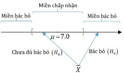
Example 6.2 Survey on the average score of students after graduation, of a faculty, of a university. We want to know if the average score of students is different from 7.0. Then the hypothesis and the opposite are as follows:

Hypothesis H 0 :  7.0 Equivalent H 1 :  7.0

The testing was done by surveying 100 students about their average score. And calculating

The average score of a student, the value is X. Because we are comparing the sample mean and the overall mean  7.0 , so the comparison must be within an allowable error. With that error

we open a range of values around  7.0 . If X is not in that region, we reject the hypothesis  H 0 , that is, the opposite  H 1true, otherwise we do not have enough evidence to reject  H 0 . The diagram is as follows:

6.1.2 Type I error and type II error.

The decisions for the model will consist of true and false outcomes given by the following table:

The hypothetical reality is not

Decision

Correct	Wrong
Reject H 0	Type I error:  	Right decision
Accept H 0	Right decision	Type II error  

Maybe you are interested!

Type I error : Reject H 0when in fact H 0true. The probability of making a type I error is denoted by the symbol  .

Type II error : Accept H 0when in fact H 0false. The probability of making a type II error is denoted by the symbol  .

The appropriateness of a statistical test is measured by the probability of making a type I error and a type II error. Because  is the probability of rejecting H 0When in fact this hypothesis is true, this is a measure of the chance of falsely rejecting H 0. Because  is the probability of accepting H 0When

In fact this hypothesis is false, so its complement, 1  is the probability of rejecting H 0 when

This hypothesis is false. Probability 1  is called the power of the model's test .

Another way to report the test results is through the p-value . The probability  of making a type I error is often called the significance level of the test model, and during the test we can choose different significance levels (for example  0.05 z /2 1.96 ,

 0.01 z /2 2.58 ,…) so sometimes the test result rejects at the first significance level, but accepts at the second significance level. So sometimes the reports will choose the lowest significance level for the test model to be meaningful.

The observed p -value or significance level is the smallest value of  for which the test models

statistically significant

If a test result is statistically significant with  0.10 but not significant with

 0.05 then we can understand the p value as a number in the range 0.05 p 0.10 . In other words, if the p value is less than the  value , then we reject the hypothesis H 0and vice versa.

6.2. HYPOTHESIS TESTING FOR A POPULATION PROPORTION VALUE.

6.2.1 Analysis.

Consider a population and a characteristic A , each element in the population has only two properties: it has property A or it does not have property A. Considering a specific data sample, we need to test the hypothesis that the proportion of type A elements in this population is p , then p is equal to the value p 0given or not with significance level  .

Observe each element and see if the observed element has property A or not. Do the job.

n times, respectively is the data sample. Let X be the random variable indexing the element with property A

, combining the assumption p p 0 we have (according to chapters 3 and 6) we have:

np 0 1p 0

X ~ N  np , np  1 p  z 

X np 0

~ N  0;1 

o 0 0

Let f be the proportion of elements with property A in n observed elements. We have

z X np 0

X p

np 0  1 p 0 

n 0 

np 0  1 p 0 

f p 0

p 0  1 p 0 

n ~ N  0;1 

The z value is a measure of the difference between f (the proportion of elements with property A in the data sample, represented by p ) and p 0.

In the test problem with the hypothesis H 0: p p 0and the opposite H 1: p p 0.

The significance level  is equally divided between the two sides and P  z z /2   : is the probability of deciding to reject the hypothesis H 0when in fact the hypothesis H 0correct.

That is, we accept the covariance H 1 when z  z  /2 or

z z  /2

In the test problem with the hypothesis H 0: p p 0and the opposite H 1: p p 0.

The significance level α is right-sided and P zz   : is the probability of deciding to reject the hypothesis H 0when in fact the hypothesis H 0correct.

That is, we accept the contradiction H 1 when z z 

In the test problem with the hypothesis H 0: p p 0and the opposite H 1: p p 0.

The significance level α is right-sided and P z z   : is the probability of deciding to reject the hypothesis H 0when in fact the hypothesis H 0correct.

That is, we accept the covariance H 1 when z  z 

1. Null hypothesis H 0 : p p 0

2. Hypothesis

3. Statistical value

Where f is the proportion of elements with characteristic A in the sample. The statistical value is: z 

4. Rejection Domain

6.2.2 Testing model.

Two-sided testing

One-sided test

H 1 : p p 0

H 1 : p p 0

H 1 : p p 0

f p 0 p 0  1 p 0 

Two-sided testing

Parallelism : H 1 : p p 0

Reject H 0 when:

 z  z  /2

  z z z z /2

 /2

One-sided inspection

Opposite : H 1 : p p 0

Reject H 0 when:

z  z  /2

One-sided inspection

Opposite : H 1 : p p 0

Reject H 0 when:

z z 

f p 0 p 0  1 p 0 

Example 6.3 Previous reports of a survey of the family background of freshmen at a university reported that 86% of first-year university students had some financial support. This year, the university conducted a similar survey on the same issue, asking 1,000 randomly selected freshmen and found that 890 students received financial support from their families. With a significance level of  5% , are the above reports still true for this year's student situation?

Solution. The testing model in this case has the form

H 0 : p 86% and H 1 : p 86%

Where p is the proportion of freshmen receiving financial aid from their families.

And the given data is: n 1000 and f 890 0.89

1000

The statistic used in this model is z 

In which p 0 0.86 so we have z 2,734

The significance level of the test is 5% corresponding to the z percentile  /2  1.96 .

Conclusion : because the statistical value is higher than the z- percentilez /2  so we can completely reject the hypothesis H 0, that is

The percentage of freshmen this year receiving financial aid from their families is different than reported in previous years.

6.3. HYPOTHESIS TESTING FOR A POPULATION MEAN.

6.3.1 Analysis.

Consider a population, let  be the average value of the population, based on a specific sample we need to check

assume that the population mean is equal to the value  0given zero with significance level  .

Let X be a random variable indicating the value of an element in the population, assuming X has a normal distribution law X ~ N   ;  2 ,  2is the population variance. Consider a data sample, with sample size n and mean

of the sample is X , (according to chapter 5) we have X ~ N  ;  2 . Combining the assumption  

, put:

n 0



z  X    X   0

2



n ~ N  0;1 

The value of z measures the difference between the sample mean (represented by  ) and the null hypothesis test model H 0:   0.

 0, is the statistical value

In case the total variance is unknown, we replace the total variance with the

n 1

 n 1  S 2

 2

sample error  S 2 . Set:

z  X   X  . 1 X  .

X 

~ 

 n 1  S 2

S



X 

In there

 ~ N  0;1  and

 2 n  1

so z 

n ~ t  n  1 

But when the sample size is larger than 30, the Student's t-test is approximately equal to the normal distribution. So when the method

unknown population error and sample size n 30 , we have:

z  X  

n ~ N  0;1 

Two-sided testing

One-sided test

H 1 :   0

H 1 :   0

H 1 :   0

6.3.2 Compare the overall mean with a number when the variance is known.

1. Null hypothesis H 0 :   0 .

2. Alternative hypothesis.

3. Statistical value

Statistical value: z X  0n



4. Rejection Domain

Two-sided testing

Equivalent : H 1 :   0

Reject H 0 when:

 z  z  /2

  z z

 /2

One-sided inspection

Equivalent: H 1 :   0

Reject H 0 when:

z  z 

One-sided inspection

Parallelism: H 1 :   0

Reject H 0 when:

z z 

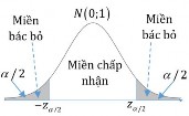
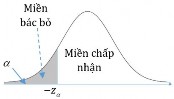
1. Null hypothesis H 0:   0.

2. Alternative hypothesis.

3. Statistical value

Statistical value: z X  0n

4. Rejection Domain

a. Case of sample size n 30, statistical value has normal distribution: z~ N  0;1  .

6.3.3 Comparing a population mean with a number when the variance is unknown.

Two-sided testing

One-sided test

H 1 :   0

H 1 :   0

H 1 :   0

S / n

Two-sided testing

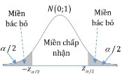
Equivalent : H 1 :   0

Reject H 0 when:

 z  z  /2

  z z

 /2

One-sided inspection

Equivalent: H 1 :   0

Reject H 0 when:

z  z 

1 fee inspection

Parallelism: H 1 :   0

Reject H 0 when:

z z 

b. Case where sample size n 30, statistical value has Student distribution, degrees of freedom

 n  1 : z ~ t  n  1  .

2-way inspection 1-fee inspection 1-way inspection

Equivalent : H 1 :   0 Equivalent : H 1 :   0 Opposite : H 1 :   0

Reject H 0 when : Reject H 0 when :

 z  t n  1 z  t n  1 z tn  1

 /2  

  z tn  1

 /2

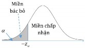
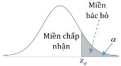
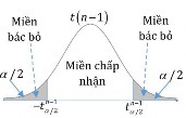
Example 6.4 Daily output at a chemical plant, recorded for n 50 days, there is a sample mean and standard deviation X 871 tons and S 21 tons. Test the hypothesis that the average daily output of the factory is  880 tons per day versus the alternative hypothesis of  either greater or less than 880 tons per day.

Prize:

Testing model:

1. H 0 :  880 tons and H 1 :  880 tons

Where  is the average output of the chemical plant in one day.

2. Statistical value: z X  0

In which X 871;  880; S 21; n 50 , so we have z  3.03

With  0.05 ; we have z  /2 1.96

Conclusion: because z z /2 so we reject the hypothesis H 0; that is  880 tons is wrong.

Example 6.5 A survey of tuna catches in a certain area of the ocean over the past year reported that the average weight of a tuna in previous years was approximately 30.31 pounds.

 1 pound 0.453592kg . But recently tuna fishing has increased, affecting the importance of

Average weight of a tuna in the area, survey sample of 20 fish gives the following data table:

17.4

18.9	39.6	34.4	19.6	24.1	39.6	12.2	25.5	22.1
33.7	37.2	43.4	41.7	27.5	29.3	21.1	23.8	43.2	24.4

Ask whether the above data sample is strong enough to reject the above argument with significance level  5%

Solution. The corresponding testing model for the problem is: 1. H 0 :  30,31 and H 1 :  30.31

Where  is the average weight of a tuna caught in this sea area.

2. Statistical value of the model: (small sample size n )20 ; total variance unknown) :

z X  0

With the obtained data we have n 20 ; X 28,935 ; S 9.5074 . So we have the value of the statistic:

z  0.6468 .

With significance level  5% we have the percentile using t n  1 t 192,093 .

 /2 0.025

Conclusion z t 19 so there is not enough evidence to reject the null hypothesis H , that is, the mean weight

0.025

The average weight of a tuna in these waters is still 30.31 pounds.

6.4. HYPOTHESIS TESTING FOR THE TOTAL VARIANCE.

6.4.1 Analysis

Overall, let  2is the variance of the population, based on a specific data sample, we need to test the hypothesis that the population variance is equal to the value  2given or not with significance level  .

In the case where the population knows the mean value is  and combines the hypothesis H :  2  2. With sample

0 0

data in turn receives the value X iwith i 1, n , we have



X ~ N   ,  2 X i  ~ N  0;1 with i 1, n .

i 0

According to the definition of Chi-square distribution we have:

  X i 

 i  1 ~  2



2 n

Thus  is the statistical value in the hypothesis testing model H :  2  2, with the law of distribution

0 0

Chi squared degrees of freedom n .

In the case where the population mean is unknown, with S 2 being the sample variance of the data, the pseudo-match

set H :  2   2 , in Chapter 5 we have:

0 0

 n 1  S 2



 2

~ 

n  1

And we have  now as the statistical value for the test model H :  2  2, when the average is unknown

0 0

overall, and has a Chi-square distribution with degrees of freedom  n  1 .

Null hypothesis H :  2  2 .

Assume alternative.

3. Statistical value.

6.4.2 Compare the overall variance with a number when the mean µ is known.

Two-sided testing

One-sided test
H :  2  2	H :  2   2
1 0	1 0
	H :  2   2
	1 0

With  : overall average.

  x   2

Statistical value:  i  1

 2

4. Rejection domain.

The statistical value has a Chi-square distribution with degrees of freedom n :  ~  2

Two-sided testing

Correspondence: H :  2  2

1 0

Reject H 0 when:

  n

1   /2

   n

 /2

1 fee inspection

Correspondence: H :  2  2

1 0

Reject H 0 when:

  n

1  

One-sided inspection

Correspondence: H :  2  2

1 0

Reject H 0 when:

  n



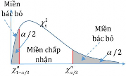
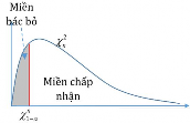
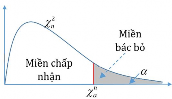
Two-sided testing	One-sided test
H :  2  2	H :  2  2
1 0	1 0
	H :  2   2
	1 0

6.4.3 Comparing the overall variance with a number when the mean µ is unknown.

1. Null hypothesis H :  2  2 .

0 0

2. Alternative hypothesis.

3. Statistical value. With

 n  1  S 2

Statistical value:   2

4. Rejection domain.

The statistical value has a Chi-square distribution with degrees of freedom  n  1 :  ~  2

n  1

Two-sided testing

Correspondence: H :  2  2

1 0

Reject H 0 when:

  n  1

1   /2

   n  1

 /2

One-sided inspection

Congruence: H :  2   2

1 0

Reject H 0 when:

  n  1

1  

One-sided inspection

Correspondence: H :  2   2

1 0

Reject H 0 when:

  n  1



Comment