Testing the Robustness of a 1-Lag Var Model

The experimental research results of Driffill and Rotondi (2007) show that the inertia of CSTT according to Taylor rule for the experimental sample is 0.6 to 0.77 as presented in the introduction of the thesis.

- Considering the period 2000Q1 – 2007Q4: most of the variables have regression coefficients β π , β y that are not statistically significant, because this period of interest rate liberalization, the interest rate of the State Bank is only indicative. The interest rate smoothing coefficient (ρ) is quite high, showing that the influence of the previous period's interest rate strongly affects the current period's interest rate. During this period, the State Bank's interest rates do not follow the Taylor rule.

- Considering the period 2008Q1 – 2015Q4: the regression results show that most of the variables have statistically significant regression coefficients, except for the output deviation coefficients β y of the variables LSTCK and LSTCV. The regression coefficients are all positive and the smoothing coefficient revolves around the value of 0.6. LSTN calculated from the Taylor rule (r*) of the variable TLS is larger than LSTN (r* VN ), showing that during this period, the State Bank focused on the target of controlling inflation. The regression results can conclude that the State Bank's interest rate during this period followed the Taylor rule in the form of an interest rate smoothing model.

- Considering the whole period and each period, among all interest rate variables, TLS gives the LSTN value (r*) closest to the average real interest rate value (r* VN ) and the regression result from the Taylor rule model of interest rate smoothing with lag equal to 1 is consistent with the actual interest rate policy of the State Bank of Vietnam in the period 2000 - 2015, in which TLS is most consistent with the Taylor rule, reflecting the same results as the results calculated from the conventional method without regression according to the original Taylor model (1993).

To further explore the interactions between interest rate, inflation and output variables, the author uses a VAR model to consider the lag of the effects and variance decomposition to see the depth of interactions between these variables.

3.2.2.3 Interest rate policy analysis using VAR model

a. Choosing the optimal lag of the model

Variables entered into the VAR model must be stationary.

Select the appropriate lag by comparing the evaluation criteria LR, PPE, AIC, SC and HQ.

Determine the stability of the model (stability test) through examining the roots of the autoregressive model (AR roots table/graph). If the roots lie within the unit circle, it proves that the VAR model is stable and vice versa.

As determined in section 3.2.2.1 Table 3.5, the variables INF, OGAP, and TLS are stationary at the 1%, 5%, and 10% significance levels.

Using Eviews 6.0 software with 3-variable VAR model TLS, INF and OGAP, we have the results of lag selection shown in Table 3.10.

Table 3.10: Lag selection of VAR model

VAR Lag Order Selection Criteria

Endogenous variables: TLS INF OGAP
Exogenous variables: C
Sample: 2000Q1 2015Q4
Included observations: 60
Lag	LogL	LR	FPE	AIC	SC	HQ
0	-373.135	NA	55.9362	12.53783	12.64255	12.57879
1	-259.6709	211.7997	1.720576	9.055696	9.474565*	9.219539
2	-242.0276	31.16976	1.29325	8.767587	9.500608	9.054312
3	-227.348	24.46609*	1.076862*	8.578266*	9.625438	8.987872*
4	-219.6464	12.06582	1.13752	8.621546	9.98287	9.154035
* indicates lag order selected by the criterion
LR: sequential modified LR test statistic (each test at 5% level)
FPE: Final prediction error
AIC: Akaike information criterion
SC: Schwarz information criterion
HQ: Hannan-Quinn information criterion

Maybe you are interested!

• Perfecting the interest rate management mechanism of the State Bank of Vietnam in the conditions of a market economy - 30
• Qos Assurance Methods for Multimedia Communications zt2i3t4l5ee zt2a3gs zt2a3ge zc2o3n4t5e6n7ts low. The EF PHB requires a sufficiently large number of output ports to provide low delay, low loss, and low jitter. EF PHBs can be implemented if the output port's bandwidth is sufficiently large, combined with small buffer sizes and other network resources dedicated to EF packets, to allow the router's service rate for EF packets on an output port to exceed the arrival rate λ of packets at that port. This means that packets with PHB EF are considered with a pre-allocated amount of output bandwidth and a priority that ensures minimum loss, minimum delay and minimum jitter before being put into operation. PHB EF is suitable for channel simulation, leased line simulation, and real-time services such as voice, video without compromising on high loss, delay and jitter values. Figure 2.10 Example of EF installation Figure 2.10 shows an example of an EF PHB implementation. This is a simple priority queue scheduling technique. At the edges of the DS domain, EF packet traffic is prioritized according to the values ​​agreed upon by the SLA. The EF queue in the figure needs to output packets at a rate higher than the packet arrival rate λ. To provide an EF PHB over an end-to-end DS domain, bandwidth at the output ports of the core routers needs to be allocated in advance to ensure the requirement μ > λ. This can be done by a pre-configured provisioning process. In the figure, EF packets are placed in the priority queue (the upper queue). With such a length, the queue can operate with μ > λ. Since EF was primarily used for real-time services such as voice and video, and since real-time services use UDP instead of TCP, RED is generally not suitable for EF queues because applications using UDP will not respond to random packet drop and RED will strip unnecessary packets. 2.2.4.2 Assured Forwarding (AF) PHB PHB AF is defined by RFC 2597. The purpose of PHB AF is to deliver packets reliably and therefore delay and jitter are considered less important than packet loss. PHB AF is suitable for non-real-time services such as applications using TCP. PHB AF first defines four classes: AF1, AF2, AF3, AF4. For each of these AF classes, packets are then classified into three subclasses with three distinct priority levels. Table 2.8 shows the four AF classes and 12 AF subclasses and the DSCP values ​​for the 12 AF subclasses defined by RFC 2597. RFC 2597 also allows for more than three separate priority levels to be added for internal use. However, these separate priority levels will only have internal significance. PHB Class PHB Subclass Package type DSCP AF4 AF41 Short 100010 AF42 Medium 100100 AF43 High 100110 AF3 AF31 Short 011010 AF32 Medium 011100 AF33 High 011110 AF2 AF21 Short 010010 AF22 Medium 010100 AF23 High 010110 AF1 AF11 Short 001010 AF12 Medium 001100 AF13 High 001110 Table 2.8 AF DSCPs The AF PHB ensures that packets are forwarded with a high probability of delivery to the destination within the bounds of the rate agreed upon in an SLA. If AF traffic at an ingress port exceeds the pre-priority rate, which is considered non-compliant or “out of profile”, the excess packets will not be delivered to the destination with the same probability as the packets belonging to the defined traffic or “in profile” packets. When there is network congestion, the out of profile packets are dropped before the in profile packets are dropped. When service levels are defined using AF classes, different quantity and quality between AF classes can be realized by allocating different amounts of bandwidth and buffer space to the four AF classes. Unlike EF, most AF traffic is non-real-time traffic using TCP, and the RED queue management strategy is an AQM (Adaptive Queue Management) strategy suitable for use in AF PHBs. The four AF PHB layers can be implemented as four separate queues. The output port bandwidth is divided into four AF queues. For each AF queue, packets are marked with three “colors” corresponding to three separate priority levels. In addition to the 32 DSCP 1 groups defined in Table 2.8, 21 DSCPs have been standardized as follows: one for PHB EF, 12 for PHB AF, and 8 for CSCP. There are 11 DSCP 1 groups still available for other standards. 2.2.5.Example of Differentiated Services We will look at an example of the Differentiated Service model and mechanism of operation. The architecture of Differentiated Service consists of two basic sets of functions: Edge functions: include packet classification and traffic conditioning. At the inbound edge of the network, incoming packets are marked. In particular, the DS field in the packet header is set to a certain value. For example, in Figure 2.12, packets sent from H1 to H3 are marked at R1, while packets from H2 to H4 are marked at R2. The labels on the received packets identify the service class to which they belong. Different traffic classes receive different services in the core network. The RFC definition uses the term behavior aggregate rather than the term traffic class. After being marked, a packet can be forwarded immediately into the network, delayed for a period of time before being forwarded, or dropped. We will see that there are many factors that affect how a packet is marked, and whether it is forwarded immediately, delayed, or dropped. Figure 2.12 DiffServ Example Core functionality: When a DS-marked packet arrives at a Diffservcapable router, the packet is forwarded to the next router based on Per-hop behavior is associated with packet classes. Per-hop behavior affects router buffers and the bandwidth shared between competing classes. An important principle of the Differentiated Service architecture is that a router's per-hop behavior is based only on the packet's marking or the class to which it belongs. Therefore, if packets sent from H1 to H3 as shown in the figure receive the same marking as packets from H2 to H4, then the network routers treat the packets exactly the same, regardless of whether the packet originated from H1 or H2. For example, R3 does not distinguish between packets from h1 and H2 when forwarding packets to R4. Therefore, the Differentiated Service architecture avoids the need to maintain router state about separate source-destination pairs, which is important for network scalability. Chapter Conclusion Chapter 2 has presented and clarified two main models of deploying and installing quality of service in IP networks. While the traditional best-effort model has many disadvantages, later models such as IntServ and DiffServ have partly solved the problems that best-effort could not solve. IntServ follows the direction of ensuring quality of service for each separate flow, it is built similar to the circuit switching model with the use of the RSVP resource reservation protocol. IntSer is suitable for services that require fixed bandwidth that is not shared such as VoIP services, multicast TV services. However, IntSer has disadvantages such as using a lot of network resources, low scalability and lack of flexibility. DiffServ was born with the idea of ​​solving the disadvantages of the IntServ model. DiffServ follows the direction of ensuring quality based on the principle of hop-by-hop behavior based on the priority of marked packets. The policy for different types of traffic is decided by the administrator and can be changed according to reality, so it is very flexible. DiffServ makes better use of network resources, avoiding idle bandwidth and processing capacity on routers. In addition, the DifServ model can be deployed on many independent domains, so the ability to expand the network becomes easy. Chapter 3: METHODS TO ENSURE QoS FOR MULTIMEDIA COMMUNICATIONS In packet-switched networks, different packet flows often have to share the transmission medium all the way to the destination station. To ensure the fair and efficient allocation of bandwidth to flows, appropriate serving mechanisms are required at network nodes, especially at gateways or routers, where many different data flows often pass through. The scheduler is responsible for serving packets of the selected flow and deciding which packet will be served next. Here, a flow is understood as a set of packets belonging to the same priority class, or originating from the same source, or having the same source and destination addresses, etc. In normal state when there is no congestion, packets will be sent as soon as they are delivered. In case of congestion, if QoS assurance methods are not applied, prolonged congestion can cause packet drops, affecting service quality. In some cases, congestion is prolonged and widespread in the network, which can easily lead to the network being "frozen", or many packets being dropped, seriously affecting service quality. Therefore, in this chapter, in sections 3.2 and 3.3, we introduce some typical network traffic load monitoring techniques to predict and prevent congestion before it occurs through the measure of dropping (removing) packets early when there are signs of impending congestion. 3.1. DropTail method DropTail is a simple, traditional queue management method based on FIFO mechanism. All incoming packets are placed in the queue, when the queue is full, the later packets are dropped. Due to its simplicity and ease of implementation, DropTail has been used for many years on Internet router systems. However, this algorithm has the following disadvantages: − Cannot avoid the phenomenon of “Lock out”: Occurs when 1 or several traffic streams monopolize the queue, making packets of other connections unable to pass through the router. This phenomenon greatly affects reliable transmission protocols such as TCP. According to the anti-congestion algorithm, when locked out, the TCP connection stream will reduce the window size and reduce the packet transmission speed exponentially. − Can cause Global Synchronization: This is the result of a severe “Lock out” phenomenon. Some neighboring routers have their queues monopolized by a number of connections, causing a series of other TCP connections to be unable to pass through and simultaneously reducing the transmission speed. After those monopolized connections are temporarily suspended, Once the queue is cleared, it takes a considerable amount of time for TCP connections to return to their original speed. − Full Queue phenomenon: Data transmitted on the Internet often has an explosion, packets arriving at the router are often in clusters rather than in turn. Therefore, the operating mechanism of DropTail makes the queue easily full for a long period of time, leading to the average delay time of large packets. To avoid this phenomenon, with DropTail, the only way is to increase the router's buffer, this method is very expensive and ineffective. − No QoS guarantee: With the DropTail mechanism, there is no way to prioritize important packets to be transmitted through the router earlier when all are in the queue. Meanwhile, with multimedia communication, ensuring connection and stable speed is extremely important and the DropTail algorithm cannot satisfy. The problem of choosing the buffer size of the routers in the network is to “absorb” short bursts of traffic without causing too much queuing delay. This is necessary in bursty data transmission. The queue size determines the size of the packet bursts (traffic spikes) that we want to be able to transmit without being dropped at the routers. In IP-based application networks, packet dropping is an important mechanism for indirectly reporting congestion to end stations. A solution that prevents router queues from filling up while reducing the packet drop rate is called dynamic queue management. 3.2. Random elimination method – RED 3.2.1 Overview RED (Random Early Detection of congestion; Random Early Drop) is one of the first AQM algorithms proposed in 1993 by Sally Floyd and Van Jacobson, two scientists at the Lawrence Berkeley Laboratory of the University of California, USA. Due to its outstanding advantages compared to previous queue management algorithms, RED has been widely installed and deployed on the Internet. The most fundamental point of their work is that the most effective place to detect congestion and react to it is at the gateway or router. Source entities (senders) can also do this by estimating end-to-end delay, throughput variability, or the rate of packet retransmissions due to drop. However, the sender and receiver view of a particular connection cannot tell which gateways on the network are congested, and cannot distinguish between propagation delay and queuing delay. Only the gateway has a true view of the state of the queue, the link share of the connections passing through it at any given time, and the quality of service requirements of the traffic flows. The RED gateway monitors the average queue length, which detects early signs of impending congestion (average queue length exceeding a predetermined threshold) and reacts appropriately in one of two ways: − Drop incoming packets with a certain probability, to indirectly inform the source of congestion, the source needs to reduce the transmission rate to keep the queue from filling up, maintaining the ability to absorb incoming traffic spikes. − Mark “congestion” with a certain probability in the ECN field in the header of TCP packets to notify the source (the receiving entity will copy this bit into the acknowledgement packet). Figure 3. 1 RED algorithm The main goal of RED is to avoid congestion by keeping the average queue size within a sufficiently small and stable region, which also means keeping the queuing delay sufficiently small and stable. Achieving this goal also helps: avoid global synchronization, not resist bursty traffic flows (i.e. flows with low average throughput but high volatility), and maintain an upper bound on the average queue size even in the absence of cooperation from transport layer protocols. To achieve the above goals, RED gateways must do the following: − The first is to detect congestion early and react appropriately to keep the average queue size small enough to keep the network operating in the low latency, high throughput region, while still allowing the queue size to fluctuate within a certain range to absorb short-term fluctuations. As discussed above, the gateway is the most appropriate place to detect congestion and is also the most appropriate place to decide which specific connection to report congestion to. − The second thing is to notify the source of congestion. This is done by marking and notifying the source to reduce traffic. Normally the RED gateway will randomly drop packets. However, if congestion If congestion is detected before the queue is full, it should be combined with packet marking to signal congestion. The RED gateway has two options: drop or mark; where marking is done by marking the ECN field of the packet with a certain probability, to signal the source to reduce the traffic entering the network. − An important goal that RED gateways need to achieve is to avoid global synchronization and not to resist traffic flows that have a sudden characteristic. Global synchronization occurs when all connections simultaneously reduce their transmission window size, leading to a severe drop in throughput at the same time. On the other hand, Drop Tail or Random Drop strategies are very sensitive to sudden flows; that is, the gateway queue will often overflow when packets from these flows arrive. To avoid these two phenomena, gateways can use special algorithms to detect congestion and decide which connections will be notified of congestion at the gateway. The RED gateway randomly selects incoming packets to mark; with this method, the probability of marking a packet from a particular connection is proportional to the connection's shared bandwidth at the gateway. − Another goal is to control the average queue size even without cooperation from the source entities. This can be done by dropping packets when the average size exceeds an upper threshold (instead of marking it). This approach is necessary in cases where most connections have transmission times that are less than the round-trip time, or where the source entities are not able to reduce traffic in response to marking or dropping packets (such as UDP flows). 3.2.2 Algorithm This section describes the algorithm for RED gateways. RED gateways calculate the average queue size using a low-pass filter. This average queue size is compared with two thresholds: minth and maxth. When the average queue size is less than the lower threshold, no incoming packets are marked or dropped; when the average queue size is greater than the upper threshold, all incoming packets are dropped. When the average queue size is between minth and maxth, each incoming packet is marked or dropped with a probability pa, where pa is a function of the average queue size avg; the probability of marking or dropping a packet for a particular connection is proportional to the bandwidth share of that connection at the gateway. The general algorithm for a RED gateway is described as follows: [5] For each packet arrival Caculate the average queue size avg If minth ≤ avg < maxth div.maincontent .s1 { color: black; font-family:"Times New Roman", serif; font-style: normal; font-weight: normal; text-decoration: none; font-size: 15pt; } div.maincontent .s2 { color: black; font-family:"Times New Roman", serif; font-style: normal; font-weight: bold; text-decoration: none; font-size: 15pt; } div.maincontent .p { color: black; font-family:"Times New Roman", serif; font-style: normal; font-weight: normal; text-decoration: none; font-size: 14pt; margin:0pt; } div.maincontent p { color: black; font-family:"Times New Roman", serif; font-style: normal; font-weight: normal; text-decoration: none; font-size: 14pt; margin:0pt; } div.maincontent .s3 { color: black; font-family:"Times New Roman", serif; font-style: normal; font-weight: bold; text-decoration: none; font-size: 14pt; } div.maincontent .s4 { color: black; font-family:"Times New Roman", serif; font-style: normal; font-weight: normal; text-decoration: none; font-size: 14pt; } div.maincontent .s5 { color: black; font-family:"Times New Roman", serif; font-style: italic; font-weight: normal; text-decoration: none; font-size: 14pt; } div.maincontent .s6 { color: black; font-family:"Times New Roman", serif; font-style: italic; font-weight: bold; text-decoration: none; font-size: 14pt; } div.maincontent .s7 { color: black; font-family:Wingdings; font-style: normal; font-weight: normal; text-decoration: none; font-size: 14pt; } div.maincontent .s8 { color: black; font-family:Arial, sans-serif; font-style: italic; font-weight: bold; text-decoration: none; font-size: 15pt; } div.maincontent .s9 { color: black; font-family:"Times New Roman", serif; font-style: normal; font-weight: bold; text-decoration: none; font-size: 14pt; } div.maincontent .s10 { color: black; font-family:"Times New Roman", serif; font-style: normal; font-weight: normal; text-decoration: none; font-size: 9pt; vertical-align: 6pt; } div.maincontent .s11 { color: black; font-family:"Times New Roman", serif; font-style: normal; font-weight: normal; text-decoration: none; font-size: 13pt; } div.maincontent .s12 { color: black; font-family:"Times New Roman", serif; font-style: normal; font-weight: normal; text-decoration: none; font-size: 10pt; } div.maincontent .s13 { color: black; font-family:"Times New Roman", serif; font-style: normal; font-weight: normal; text-d
• Applying Taylor rule in the interest rate management mechanism of the State Bank of Vietnam - 28
• Applying Taylor rule in the interest rate management mechanism of the State Bank of Vietnam - 31
• Regression Results of Bank Profitability Model from Interest Rate and Other Profit Determinants

Source: author calculated from Eviews 6.0 software

The lags recommended by Eviews are 1 (SC), and 3 (LR, HQ, FPE, AIC). As analyzed in section 2.3.1, according to Ivanov and Kilian (2005), the SC evaluation criterion with lag equal to 1 was chosen because this is a quarterly VAR model and the sample size is less than 120.

b. Testing the stability of the model

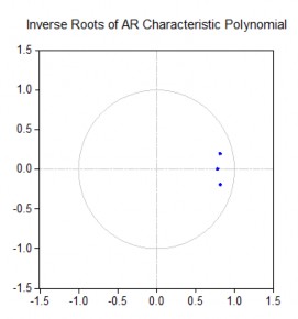
The test results presented in Table 3.11 show that there is no solution outside the unit circle, the VAR(1) model satisfies the sustainability condition.

Table 3.11: Testing the sustainability of the VAR model with lag 1

Roots of Characteristic Polynomial

	Endogenous variables: TLS INF OGAP
	Exogenous variables: C
	Lag specification: 1 1
	Root	Modulus
	0.818750 - 0.196931i	0.842101
	0.818750 + 0.196931i	0.842101
	0.786057	0.786057
	No root lies outside the unit circle.
	VAR satisfies the stability condition.

Source: results from Eviews 6.0 software

Conclusion: The VAR model is reasonable according to the variables TLS, INF and OGAP with lag 1. The VAR(1) model is also compatible with the 3-variable Taylor rule model looking back to the past with lag 1 presented in section 3.2.2.2.

c. Test of causality

Causality testing indicates whether a variable has an influence or impact on another variable. Using the Granger Causality/Block Exogeneity Wald test (GCBEW) method using Eviews 6.0 software, the results for the VAR(1) model with the variables TLS, INF and OGAP are shown in Appendix 14. When changing the lag of the VAR(p) model, the impact relationship between the variables also changes. Appendix 14 lists the results of causality testing using the VAR(p) model with p taking values ​​from 1 to 8. When p = 1, the variables INF and OGAP have an influence on the TLS variable, and at the same time, the variables TLS and OGAP also have an impact on the INF variable, however, the variables TLS and INF have no impact on the OGAP variable. When p

= 2, 3, 4, only the INF variable has an impact on the TLS variable, the TLS and OGAP variables have no impact on the INF variable, and the TLS and INF variables also have no impact on the OGAP variable. This shows that with a lag of one quarter, the TLS and INF variables have a causal relationship that affects each other, while the output deviation variable

OGAP has an impact on both TLS and INF variables but does not receive the opposite impact from TLS and INF variables. This shows that the SBV's tightening monetary policy to control inflation has an effect immediately after one quarter. With a lag from the second quarter onwards to the fourth quarter, inflation will impact TLS but there is little impact from TLS to inflation.

When p = 5, 6, 7, 8 the causal relationship between the variables is stronger with the statistical values ​​of χ 2 (All) being mostly less than the 5% significance level, indicating that in the long run the variables have a mutual impact on each other.

However, the GCEBW causality test does not indicate the extent to which one variable influences another. To determine the extent to which variables influence one another, economists often use two common testing methods: the impulse response function and variance decomposition.

d. Thrust reaction function

The results of the thrust response function analysis are as follows:

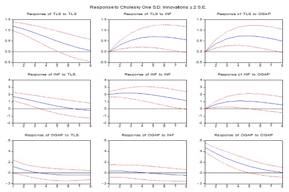
Figure 3.1: Impulse response between endogenous variables over 8 quarters (2 years)

Source: author calculated from Eviews 6.0 software

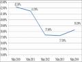
When an interest rate ceiling shock occurs, the impact on itself will gradually decrease, while the impact on inflation and output deviation increases in the first three quarters but gradually decreases in the following quarters.

When an inflation shock occurs, it has a strong impact on the interest rate ceiling and on inflation in the first three quarters and then gradually decreases; the impact on output deviation increases gradually in the first three quarters but then gradually decreases.

However, the output gap shock mainly affects itself and has little effect on inflation and interest rate ceiling in the first three quarters, then gradually decreases. The response of output gap to inflation or interest rate ceiling shock is weaker than to its own shock.

Studying the long-term impact between variables over 24 quarters (6 years) in Figure 3.2 shows that the fluctuations tend to fade after the 5th year and the variables are less responsive to shocks.

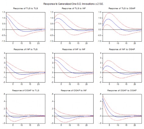
Figure 3.2: Impulse response between endogenous variables over 24 quarters (6 years)

Source: author calculated from Eviews 6.0 software

e. Variance decomposition

Variance decomposition indicates the degree of change of a given variable under the influence of shocks to that variable and shocks to other variables. Variance decomposition indicates the proportion of influence of variables on the change of a variable in the short and long run. Changing the order of variables affects the results from variance decomposition. Therefore, the order in variance decomposition is important. According to the results of the GCBEW causality test of the VAR(1) model with Taylor rule variables TLS, INF and OGAP analyzed in part (c) above, OGAP is the variable that has the least impact on the variables TLS and INF, and TLS is the target variable, so the order in the impulse response function analysis and variance decomposition will be OGAP, INF, TLS.

The variance decomposition results of the VAR(1) model with the variables TLS, INF, OGAP in the Cholesky order are OGAP, INF, TLS as follows:

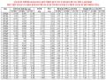
Table 3.12: Variance decomposition of VAR(1) model for the period 2000Q1 – 2015Q4

Variance decomposition of TLS variable

Quarter	Standard error (SE)	TLS	INF	OGAP
1	1,1969	56,8180	37,2688	5,9132
2	1,6762	39,2107	42.5685	18,2208
3	2,0647	27,0781	43,8833	29,0387
4	2,3902	20,2079	43,2277	36.5645
8	3.0865	16,4241	38,1229	45.4530
12	3,2098	19,1565	36,2128	44,6307
16	3.2254	19,6105	35,9574	44,4321
20	3,2343	19,5181	35,8881	44,5938
24	3,2367	19,5282	35,8552	44,6166
Variance decomposition of INF variable
Quarter	SE	TLS	INF	OGAP
1	2,6586	0.0000	95.3757	4,6243
2	3,7794	1,3682	87,4223	11,2095
3	4,6143	3,7259	79,8413	16,4328
4	5,2461	6,4541	73,6730	19,8729
8	6,3754	15,8623	61,3886	22,7491
12	6,5426	19,2749	58.7765	21,9486

16

6,5823	19.4040	58,1901	22,4060
20	6,5996	19,3239	57,9658	22,7104
24	6.6025	19,3398	57,9209	22,7393
Variance Decomposition of OGAP Variables
Quarter	SE	TLS	INF	OGAP
1	0.4902	0.0000	0.0000	100,0000
2	0.6143	0.2454	0.0626	99.6920
3	0.6711	0.6169	0.2616	99.1215
4	0.6975	0.9610	0.6346	98.4044
8	0.7203	1,3238	3,1933	95,4829
12	0.7290	1.5449	4,7416	93.7135
16	0.7325	1,9368	5,0001	93,0632
20	0.7330	2,0587	5,0021	92.9392
24	0.7331	2,0657	5,0050	92.9293
Cholesky Order: OGAP INF TLS

Source: author calculated results from Eviews 6.0 software

Table 3.12 shows that most of the impacts of the variables OGAP, INF, TLS have a major impact in the short term of three quarters, after which most of the impacts remain unchanged.

When decomposing the variance for the TLS interest rate ceiling variable, in the first quarter, the influence of INF was quite large at 37% in the variance of TLS and increased in the second and third quarters, then changed little, while OGAP accounted for a fairly small proportion of 6% and increased sharply to 18.22% in the second quarter. After that, the TLS variable gradually decreased its proportion and the OGAP variable gradually increased its proportion while the INF variable almost did not change its proportion after the third quarter. This proves that the relationship between inflation and the interest rate ceiling is strong in the short term and the interest rate policy will take effect right in the first quarter.

The variance decomposition of the INF variable shows that its proportion is quite large and gradually decreases over time, the proportion of the TLS variable increases gradually when the proportion of INF decreases, showing an inverse relationship between the two variables when the TLS factor increases, causing INF to decrease, while the proportion of the output deviation variable changes very little after the fourth quarter.

The OGAP variable difference decomposition shows that the change of this variable is mostly due to its internal influence, the impact from the two variables TLS interest rate ceiling and INF inflation is small.

This may imply that economic growth stimulation has little impact from monetary policy through interest rate tools.

Variance decomposition analysis shows more clearly the impact of variables on the change of each variable. The interaction between inflation and interest rate ceiling is relatively strong and effective in the short term, so basically controlling high inflation through interest rate policy is effective in the short term. The State Bank should effectively use the interest rate policy tool with appropriate interest rates to achieve the desired inflation target in the short term.

3.2.2.4 Optimal monetary policy: minimizing the loss function

The optimal monetary policy that central banks aim for is to determine the inflation coefficients and output deviation coefficients so that the value of the loss function is the smallest. Central banks often face the possibility of trade-offs between balancing short-term interest rate fluctuations and short-term output fluctuations, so determining the optimal inflation coefficients and output deviation coefficients helps monetary policy makers to better apply the Taylor rule in making decisions on the level of interest rates. In model (3.1), the original Taylor rule (1993) with inflation coefficients (0.5) and output deviation coefficients (0.5) is consistent with the macroeconomic data in Vietnam analyzed in section 3.2.1. However, is this the optimal coefficient of monetary policy in Vietnam?

Using quarterly macroeconomic data in Vietnam during the period 2000Q1 – 2015Q4 with the assumption that the LSTN level is 3.61%, the target inflation rate is 5%, π t is the inflation rate of the previous 4 quarters (INF), y t is the output deviation (OGAP), i t is the interest rate ceiling variable (TLS), when putting the predetermined values ​​of the coefficient pair (β π , β y ) from 0.1 to 1.5 with a step of 0.1 into the Taylor rule (1.4) to calculate the corresponding TLS value; estimate the inflation rate according to formula (2.4), and estimate the output deviation according to formula (2.5). Using Eviews 6.0 software to calculate the simulated values ​​of variables π t , y t , and i t TAYLOR when changing the value of the coefficient pair (β π , β y ), and calculating the loss function value according to formulas (2.20), (2.24) and (2.25), we have the following random simulation method results: