* Consider the case of a reverse wave from B to A (Figure 14-5,a):
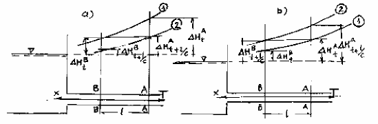
Figure 14-5. Diagram of establishing the equation of the water wave chain.
Maybe you are interested!
-
 Car body electrical practice - 8
zt2i3t4l5ee
zt2a3gs
zt2a3ge
zc2o3n4t5e6n7ts
If the voltage is out of specification, replace the wire or connector.
If the voltage is within specification, install the front fog light relay and follow step 5.
Step 5 Check the front fog light switch
- Remove the D4 connector of the fog light switch
- Use a multimeter to measure the resistance of the front fog light switch.
Measurement location
Condition
Standard
D4-3 (BFG) -D4-4 (LFG)
Light switchFront Fog OFF
>10kΩ
D4-3 (BFG) -D4-4 (LFG)
Front fog light switchON
<1 Ω
- Standard resistor
D4 connector is located on the combination switch assembly.
If the resistance is out of specification, replace the combination switch (the fog light switch is located in the combination switch).
If the resistance is within specification, follow step 6.
Step 6 Check wiring and connectors (front fog light relay-light selector switch)
- Disconnect connector D4 of the combination switch assembly
- Use a voltmeter to measure the voltage value of jack D4 on the wire side.
Measurement location
Control modecontrol
Standard
D4-3 (BFG) - (-) AQ
TAIL
11 to 14 V
D4 connector for the wiring of the combination switch assembly
If the voltage does not meet the standard, replace the wire or connector.
If the voltage is within standard, there may have been an error in the previous measurements.
Step 7 Check the front fog lights
- Remove the front fog light electrical connector.
- Supply battery voltage to the fog lamp terminals
Jack 8, B9 of front fog lamp on the electrical side
blind first.
Power supply location
Terms and Conditions
Battery positive terminal - Terminal 2Battery negative terminal - Terminal 1
Fog lightsbefore morning
- If the light does not come on, replace the bulb.
If the light is on, re-plug the jack and continue to step 8.
Step 8 Check wiring and connectors (relay and front fog lights)
- Disconnect the B8 and B9 connectors of the front fog lights.
- Use a voltmeter to measure voltage at the following locations:
Measurement location
Switch location
Terms and Conditions
B8-2 - (-) AQ
Electric lock ON TAIL size switchFog switch ON
11 to 14 V
B9-2 - (-) AQ
Electric lock ONTAIL size switch Fog switch ON
11 to 14 V
B8 and B9 connectors on the front fog lamp wiring side
Voltage is not up to standard, repair or replace the jack. If up to standard, there may have been an error in the measurement process.
2.2.4. Procedure for removing, installing and adjusting fog lights 1. Procedure for removing
- Remove the front inner ear pads
Use a screwdriver to remove the 3 screws and remove the front part of the front inner ear liner
-Remove the fog light assembly
+ Disconnect the connector.
+ Use a screwdriver to remove 3 screws to remove the fog light cover
2. Installation sequence
-Rotate the fog lamp bulb in the direction indicated by the arrow as shown in the figure and remove the fog lamp from the fog lamp assembly.
-Rotate the fog light bulb in the direction indicated by the arrow as shown in the figure and install the light into the fog light assembly.
- Use a screwdriver to install the fog light cover
-Install the electrical connector
Attention: Be careful not to damage the plastic thread on the lamp assembly.
- Install the front inner ear pads
Use a screwdriver to install the front inner bumper with 3 screws.
3. Prepare the vehicle to adjust the fog light convergence. Prepare the vehicle:
- Make sure there is no damage or deformation to the vehicle body around the fog lights.
- Add fuel to the fuel tank
- Add oil to standard level.
- Add engine coolant to standard level.
- Inflate the tire to standard pressure.
- Place spare tire, tools and jack in original design position
- Do not leave any load in the luggage compartment.
- Let a person weighing about 75 kg sit in the driver's seat.
4. Prepare to check the fog light convergence
a/ Prepare the vehicle status as follows:
- Place the car in a dark enough place to see the lines. The lines are the dividing line, below which the light from the fog lights can be seen but above which it cannot.
- Place the car perpendicular to the wall.
- Keep a distance of 7.62 m between the center of the fog lamp and the wall.
- Park the car on level ground.
- Press the car down a few times to stabilize the suspension.
Note: A distance of approximately 7.62 m is required between the vehicle (fog lamp center) and the wall to adjust the convergence correctly. If the distance of 7.62 m cannot be achieved, set the correct distance of 3 m to check and adjust the fog lamp convergence. (Since the target area varies with the distance, please follow the instructions as shown in the figure.)
b/ Prepare a piece of thick white paper about 2 m high and 4 m wide to use as a screen.
c/ Draw a vertical line through the center of the screen (line V).
d/ Set the screen as shown in the picture. Note:
- Keep the screen perpendicular to the ground.
- Align the V line on the screen with the center of the vehicle.
e/Draw the reference lines (H, V LH and V RH lines) on the screen as shown in the figure.HINT:
Mark the center of the fog lamp on the screen. If the center mark cannot be seen on the fog lamp, use the center of the fog lamp or the manufacturer's name mark on the fog lamp as the center mark.
H line (fog light height):
Draw a line across the screen so that it passes through the center mark. Line H should be at the same height as the center mark of the fog light bulb.
Line V LH, V RH (center mark position of left fog lamp LH and right fog lamp RH):
Draw two lines so that they intersect line H at the center marks.
5. Check the fog light convergence
a/ Cover the fog lamp or remove the connector of the other side fog lamp to prevent light from the unchecked fog lamp from affecting the fog lamp convergence test.
b/ Start the engine.
c/ Turn on the fog lights and make sure that the dividing line is outside the standard area as shown in the drawing.
6. Adjust the fog light convergence
Use a screwdriver to adjust the fog light to the standard area by turning the toe adjustment screw.
Note: If the screw is adjusted too far, loosen it and then tighten it again, so that the last rotation of the light adjustment screw is clockwise.
3. Self-study questions
1. Describe the operating principle of the lighting system with automatic headlight function
2. Describe the operating principle of the lighting system with the function of rotating headlights when turning
3. Draw diagram and connect lighting system on Hyundai Porter car
4. Draw diagram and connect lighting system on Honda Accord 1992
5. Draw the lighting circuit on a 1993 Toyota Lexus
LESSON 3 MAINTENANCE AND REPAIR OF SIGNAL SYSTEM
I. IMPLEMENTATION GOAL
After completing this lesson, students will be able to:
- Distinguish between types of signals on cars
- Correctly describe common symptoms and suspected areas causing damage.
- Connecting signal circuits ensures technical requirements
- Disassemble, install, check, maintain and repair the signal system to ensure technical requirements.
- Ensure safety in work and industrial hygiene
II. LESSON CONTENT
1. General description
The signal system equipped on cars aims to create signals to notify other vehicles participating in traffic about the vehicle's operating status such as: stopping, parking, braking, reversing, turning...
Signals are used either by light such as headlamps, brake lights, turn signals….. or by sound such as horns, reverse music….
Just like the lighting system. A signal system circuit usually consists of: battery, fuse, wire, relay, electrical load and control switch. Only some switches of the signal system are on the combination switch. The switches of other signals are usually located in different locations such as in the gearbox or brake pedal……
2. Maintenance and repair
2.1. Turn signals and hazard lights
The installation location of the turn signal is shown in Figure 3.1. The turn signal control switch is located in the combination switch under the steering wheel. Turning this switch to the right or left will make the turn signal turn right or left.
The hazard light switch is used when the vehicle has a problem while participating in traffic. When the hazard light switch is turned on, all the turn signals on the vehicle will light up at a certain frequency. The hazard light switch is usually placed separately from the turn signal switch (some old cars integrate the hazard and turn signal switches on the same combination switch cluster).
Figure 3.1 Turn signal switch Figure 3.2 Hazard switch
The part that generates the flashing frequency for the lights is called a turn signal relay. The turn signal relay usually has 3 terminals: B (positive power supply); E (negative power supply); L (providing the turn signal switch to distribute to the
lamp)
2.1.1. Circuit diagram
To generate the frequency for the turn signal, a turn signal relay is used in the turn signal circuit. The current from the turn signal relay will be sent to the turn signal switch assembly to distribute the current to the turn signal lights for the driver's purpose.
Figure 3.3. Schematic diagram of a turn signal circuit without a hazard switch
1. Battery; 2. Electric lock; 3. Turn signal relay; 4. Turn signal switch; 5. Turn signal lamp; 6. Turn signal lamp; 7. Hazard switch
Figure 3.4 Schematic diagram of turn signal circuit with hazard switch
1. Battery; 2. Combination switch cluster; 3. Turn signal;
4. Turn signal light; 5. Turn signal relay
Today's cars no longer use three-pin turn signal relays (B, L, E) but use eight-pin turn signal relays (figure 3.5) (pin number 8 is used for hazard lights).
For this type, the current supplying the turn signal lights is supplied directly from the turn signal relay to the lights.
div.maincontent .p { color: black; font-family:"Times New Roman", serif; font-style: normal; font-weight: normal; text-decoration: none; font-size: 14pt; margin:0pt; } div.maincontent p { color: black; font-family:"Times New Roman", serif; font-style: normal; font-weight: normal; text-decoration: none; font-size: 14pt; margin:0pt; } div.maincontent .s1 { color: black; font-family:"Times New Roman", serif; font-style: normal; font-weight: normal; text-decoration: none; font-size: 13pt; } div.maincontent .s2 { color: black; font-family:"Times New Roman", serif; font-style: italic; font-weight: normal; text-decoration: none; font-size: 14pt; } div.maincontent .s3 { color: black; font-family:"Times New Roman", serif; font-style: normal; font-weight: normal; text-decoration: none; font-size: 14pt; } div.maincontent .s4 { color: black; font-family:"Times New Roman", serif; font-style: normal; font-weight: normal; text-decoration: none; font-size: 13pt; } div.maincontent .s5 { color: black; font-family:"Times New Roman", serif; font-style: normal; font-weight: normal; text-decoration: none; font-size: 13pt; vertical-align: 1pt; } div.maincontent .s6 { color: black; font-family:"Times New Roman", serif; font-style: normal; font-weight: normal; text-decoration: none; font-size: 11pt; } div.maincontent .s7 { color: black; font-family:"Times New Roman", serif; font-style: normal; font-weight: normal; text-decoration: none; font-size: 14pt; vertical-align: -9pt; } div.maincontent .s8 { color: black; font-family:"Times New Roman", serif; font-style: normal; font-weight: normal; text-decoration: none; font-size: 11pt; } div.maincontent .s9 { color: #008000; font-family:"Times New Roman", serif; font-style: normal; font-weight: normal; text-decoration: none; font-size: 14pt; } div.maincontent .s10 { color: black; font-family:"Times New Roman", serif; font-style: italic; font-weight: normal; te
Car body electrical practice - 8
zt2i3t4l5ee
zt2a3gs
zt2a3ge
zc2o3n4t5e6n7ts
If the voltage is out of specification, replace the wire or connector.
If the voltage is within specification, install the front fog light relay and follow step 5.
Step 5 Check the front fog light switch
- Remove the D4 connector of the fog light switch
- Use a multimeter to measure the resistance of the front fog light switch.
Measurement location
Condition
Standard
D4-3 (BFG) -D4-4 (LFG)
Light switchFront Fog OFF
>10kΩ
D4-3 (BFG) -D4-4 (LFG)
Front fog light switchON
<1 Ω
- Standard resistor
D4 connector is located on the combination switch assembly.
If the resistance is out of specification, replace the combination switch (the fog light switch is located in the combination switch).
If the resistance is within specification, follow step 6.
Step 6 Check wiring and connectors (front fog light relay-light selector switch)
- Disconnect connector D4 of the combination switch assembly
- Use a voltmeter to measure the voltage value of jack D4 on the wire side.
Measurement location
Control modecontrol
Standard
D4-3 (BFG) - (-) AQ
TAIL
11 to 14 V
D4 connector for the wiring of the combination switch assembly
If the voltage does not meet the standard, replace the wire or connector.
If the voltage is within standard, there may have been an error in the previous measurements.
Step 7 Check the front fog lights
- Remove the front fog light electrical connector.
- Supply battery voltage to the fog lamp terminals
Jack 8, B9 of front fog lamp on the electrical side
blind first.
Power supply location
Terms and Conditions
Battery positive terminal - Terminal 2Battery negative terminal - Terminal 1
Fog lightsbefore morning
- If the light does not come on, replace the bulb.
If the light is on, re-plug the jack and continue to step 8.
Step 8 Check wiring and connectors (relay and front fog lights)
- Disconnect the B8 and B9 connectors of the front fog lights.
- Use a voltmeter to measure voltage at the following locations:
Measurement location
Switch location
Terms and Conditions
B8-2 - (-) AQ
Electric lock ON TAIL size switchFog switch ON
11 to 14 V
B9-2 - (-) AQ
Electric lock ONTAIL size switch Fog switch ON
11 to 14 V
B8 and B9 connectors on the front fog lamp wiring side
Voltage is not up to standard, repair or replace the jack. If up to standard, there may have been an error in the measurement process.
2.2.4. Procedure for removing, installing and adjusting fog lights 1. Procedure for removing
- Remove the front inner ear pads
Use a screwdriver to remove the 3 screws and remove the front part of the front inner ear liner
-Remove the fog light assembly
+ Disconnect the connector.
+ Use a screwdriver to remove 3 screws to remove the fog light cover
2. Installation sequence
-Rotate the fog lamp bulb in the direction indicated by the arrow as shown in the figure and remove the fog lamp from the fog lamp assembly.
-Rotate the fog light bulb in the direction indicated by the arrow as shown in the figure and install the light into the fog light assembly.
- Use a screwdriver to install the fog light cover
-Install the electrical connector
Attention: Be careful not to damage the plastic thread on the lamp assembly.
- Install the front inner ear pads
Use a screwdriver to install the front inner bumper with 3 screws.
3. Prepare the vehicle to adjust the fog light convergence. Prepare the vehicle:
- Make sure there is no damage or deformation to the vehicle body around the fog lights.
- Add fuel to the fuel tank
- Add oil to standard level.
- Add engine coolant to standard level.
- Inflate the tire to standard pressure.
- Place spare tire, tools and jack in original design position
- Do not leave any load in the luggage compartment.
- Let a person weighing about 75 kg sit in the driver's seat.
4. Prepare to check the fog light convergence
a/ Prepare the vehicle status as follows:
- Place the car in a dark enough place to see the lines. The lines are the dividing line, below which the light from the fog lights can be seen but above which it cannot.
- Place the car perpendicular to the wall.
- Keep a distance of 7.62 m between the center of the fog lamp and the wall.
- Park the car on level ground.
- Press the car down a few times to stabilize the suspension.
Note: A distance of approximately 7.62 m is required between the vehicle (fog lamp center) and the wall to adjust the convergence correctly. If the distance of 7.62 m cannot be achieved, set the correct distance of 3 m to check and adjust the fog lamp convergence. (Since the target area varies with the distance, please follow the instructions as shown in the figure.)
b/ Prepare a piece of thick white paper about 2 m high and 4 m wide to use as a screen.
c/ Draw a vertical line through the center of the screen (line V).
d/ Set the screen as shown in the picture. Note:
- Keep the screen perpendicular to the ground.
- Align the V line on the screen with the center of the vehicle.
e/Draw the reference lines (H, V LH and V RH lines) on the screen as shown in the figure.HINT:
Mark the center of the fog lamp on the screen. If the center mark cannot be seen on the fog lamp, use the center of the fog lamp or the manufacturer's name mark on the fog lamp as the center mark.
H line (fog light height):
Draw a line across the screen so that it passes through the center mark. Line H should be at the same height as the center mark of the fog light bulb.
Line V LH, V RH (center mark position of left fog lamp LH and right fog lamp RH):
Draw two lines so that they intersect line H at the center marks.
5. Check the fog light convergence
a/ Cover the fog lamp or remove the connector of the other side fog lamp to prevent light from the unchecked fog lamp from affecting the fog lamp convergence test.
b/ Start the engine.
c/ Turn on the fog lights and make sure that the dividing line is outside the standard area as shown in the drawing.
6. Adjust the fog light convergence
Use a screwdriver to adjust the fog light to the standard area by turning the toe adjustment screw.
Note: If the screw is adjusted too far, loosen it and then tighten it again, so that the last rotation of the light adjustment screw is clockwise.
3. Self-study questions
1. Describe the operating principle of the lighting system with automatic headlight function
2. Describe the operating principle of the lighting system with the function of rotating headlights when turning
3. Draw diagram and connect lighting system on Hyundai Porter car
4. Draw diagram and connect lighting system on Honda Accord 1992
5. Draw the lighting circuit on a 1993 Toyota Lexus
LESSON 3 MAINTENANCE AND REPAIR OF SIGNAL SYSTEM
I. IMPLEMENTATION GOAL
After completing this lesson, students will be able to:
- Distinguish between types of signals on cars
- Correctly describe common symptoms and suspected areas causing damage.
- Connecting signal circuits ensures technical requirements
- Disassemble, install, check, maintain and repair the signal system to ensure technical requirements.
- Ensure safety in work and industrial hygiene
II. LESSON CONTENT
1. General description
The signal system equipped on cars aims to create signals to notify other vehicles participating in traffic about the vehicle's operating status such as: stopping, parking, braking, reversing, turning...
Signals are used either by light such as headlamps, brake lights, turn signals….. or by sound such as horns, reverse music….
Just like the lighting system. A signal system circuit usually consists of: battery, fuse, wire, relay, electrical load and control switch. Only some switches of the signal system are on the combination switch. The switches of other signals are usually located in different locations such as in the gearbox or brake pedal……
2. Maintenance and repair
2.1. Turn signals and hazard lights
The installation location of the turn signal is shown in Figure 3.1. The turn signal control switch is located in the combination switch under the steering wheel. Turning this switch to the right or left will make the turn signal turn right or left.
The hazard light switch is used when the vehicle has a problem while participating in traffic. When the hazard light switch is turned on, all the turn signals on the vehicle will light up at a certain frequency. The hazard light switch is usually placed separately from the turn signal switch (some old cars integrate the hazard and turn signal switches on the same combination switch cluster).
Figure 3.1 Turn signal switch Figure 3.2 Hazard switch
The part that generates the flashing frequency for the lights is called a turn signal relay. The turn signal relay usually has 3 terminals: B (positive power supply); E (negative power supply); L (providing the turn signal switch to distribute to the
lamp)
2.1.1. Circuit diagram
To generate the frequency for the turn signal, a turn signal relay is used in the turn signal circuit. The current from the turn signal relay will be sent to the turn signal switch assembly to distribute the current to the turn signal lights for the driver's purpose.
Figure 3.3. Schematic diagram of a turn signal circuit without a hazard switch
1. Battery; 2. Electric lock; 3. Turn signal relay; 4. Turn signal switch; 5. Turn signal lamp; 6. Turn signal lamp; 7. Hazard switch
Figure 3.4 Schematic diagram of turn signal circuit with hazard switch
1. Battery; 2. Combination switch cluster; 3. Turn signal;
4. Turn signal light; 5. Turn signal relay
Today's cars no longer use three-pin turn signal relays (B, L, E) but use eight-pin turn signal relays (figure 3.5) (pin number 8 is used for hazard lights).
For this type, the current supplying the turn signal lights is supplied directly from the turn signal relay to the lights.
div.maincontent .p { color: black; font-family:"Times New Roman", serif; font-style: normal; font-weight: normal; text-decoration: none; font-size: 14pt; margin:0pt; } div.maincontent p { color: black; font-family:"Times New Roman", serif; font-style: normal; font-weight: normal; text-decoration: none; font-size: 14pt; margin:0pt; } div.maincontent .s1 { color: black; font-family:"Times New Roman", serif; font-style: normal; font-weight: normal; text-decoration: none; font-size: 13pt; } div.maincontent .s2 { color: black; font-family:"Times New Roman", serif; font-style: italic; font-weight: normal; text-decoration: none; font-size: 14pt; } div.maincontent .s3 { color: black; font-family:"Times New Roman", serif; font-style: normal; font-weight: normal; text-decoration: none; font-size: 14pt; } div.maincontent .s4 { color: black; font-family:"Times New Roman", serif; font-style: normal; font-weight: normal; text-decoration: none; font-size: 13pt; } div.maincontent .s5 { color: black; font-family:"Times New Roman", serif; font-style: normal; font-weight: normal; text-decoration: none; font-size: 13pt; vertical-align: 1pt; } div.maincontent .s6 { color: black; font-family:"Times New Roman", serif; font-style: normal; font-weight: normal; text-decoration: none; font-size: 11pt; } div.maincontent .s7 { color: black; font-family:"Times New Roman", serif; font-style: normal; font-weight: normal; text-decoration: none; font-size: 14pt; vertical-align: -9pt; } div.maincontent .s8 { color: black; font-family:"Times New Roman", serif; font-style: normal; font-weight: normal; text-decoration: none; font-size: 11pt; } div.maincontent .s9 { color: #008000; font-family:"Times New Roman", serif; font-style: normal; font-weight: normal; text-decoration: none; font-size: 14pt; } div.maincontent .s10 { color: black; font-family:"Times New Roman", serif; font-style: italic; font-weight: normal; te -
 Water Supply Methods and Valve Components on Turbine Pipes
 -
 Relationship Of Pf, Corresponding Air Pressure, Type And Constant Of Soil Water And Measurement Method
 -
 Classification According to the Condition of the Upstream Water Pressure Plant
 -
 Promotional Activities Used by the Company (Figure 2.3 - Appendix 2: Diagram, Drawing)
Section AA is on the turbine side, section BB is on the lake side, a distance l apart. The water pressure at the beginning of the period is line (1) which is higher than the water pressure at the end of the period - line (2) because this is the case of reverse waves, the water pressure value decreases. Head
The velocity period and water pressure value at AA are
VA , H A , at BB there are V B , H B .
tttt
t l / c
At the end of the period , the velocity and pressure of the water hitting AA are VA
A
, H
t l / c
, at BB will be:
V
B
t l / c
B
, H
t l / c
. Thus, at each cross-section, the water pressure value changes as follows:
At AA: H A
H A c ( VA V A
) (*)
t l/ c
t g t
t l/ c
At BB:
H B
H B c ( V B V B
) (**)
t l/ c
t g t
t l/ c
In the two formulas above, the right side has a minus sign because this is a reverse wave. If we omit
Through friction loss, the water is transmitted without deformation, so:
H B H A and
tt l/ c
V B V A
Transform and add the two formulas (*) and (**) together and rearrange them to get:
tt l/ c
H A H B c ( VA V B )
(14-9)
tt l/ c g t
t l / c
Equation (14-9) is the equation for retrograde wave propagation from BB to AA.
* . Consider the case of a forward wave from A to B (Figure 14-5,b):
Figure (14-5,b) is a diagram to determine the equation of the forward water wave chain. On this diagram, line (1) is lower than line (2) because this is a forward pressure increasing wave. The symbols and explanations to establish the formula are similar to the case of the reverse wave, except that the direction is reversed. There is also a change in the water pressure at each cross-section A and B as follows:
At AA:
H A H A
c ( VA V A
) (*')
t l / ct
g tt l / c
At BB: H B H B c ( V B V B
) (**')
t l/ct gt
t l/ c
In the two formulas above, the right side has a plus sign because this is a forward wave. Also omit
Through friction loss, the water is transmitted without deformation, so:
H A H B and
tt l/ c
V A V B
. Transform and add the two formulas (*') and (**') together and rearrange them to get
tt l/ c
The forward wave propagation equation (14-10) from AA to BB is as follows:
H B H A
( V B V A
) (14-10)
c
tt l / c
g tt l / c
b. Indirect water wave equation, relative value
For ease of calculation, the absolute water impact values (14-9) and (14-10) are converted to relative water impact values (dimensionless) in the following way:
Set H
H 0
called relative water pressure value; H 0 is the static water column without water impact;
VQ
v q
is the relative velocity and flow;
V max
c Q max
2g H 0 F
Q max
cV max
2g H 0
is the pipeline inertia coefficient.
Divide both sides of equations (14-9) and (14-10) by
H 0 and the right side multiplied by
score
V max , finally by placing the dimensionless quantities above we have the equation
V max
The relative values for the two cases of water wave propagation are as follows:
- Equation of retrograde wave transmission from B to A:
A B 2 ( v A v B )
(11-14)
tt l / ctt l / c
- Equation of forward wave transmission from A to B:
B A 2 ( v B v A )
(14-12)
tt l / ctt l / c
General application to the transmission of wave chains on pipelines,
The half-water phase difference is
= l/c. So we have the system of equations for chain wave propagation
Indirect water flow, as follows, is written for any t = n (with n = 0, 1, 2, .., ...):
n
n
v
B
Reverse wave propagation: A
B
(n 1)
2 ( v A
(n 1) )
(14-13)
Forward wave transmission:
THREE
n (n 1)
2 ( v B
(n 1) )
(14-14)
n
v
A
Equations (14-13) and (14-14) are called wave propagation equations, or chain equations because based on them we can determine the water pressure values at successive half-phases when knowing the boundary conditions and initial conditions.
XIV. 2. 2. Calculation of water impact by analytical method
The absolute or relative water wave propagation equations can be used in combination with boundary conditions or initial conditions to calculate the water pressure. Here we present how to use the relative wave propagation equations (14-13) and (14-14) to calculate with two methods: analytical and graphical. In this section we use the analytical method to solve.
1. Boundary conditions and initial conditions
To solve the water impact problem by analytical method, we first determine the
Boundary conditions and initial conditions at two cross sections AA and BB of the pipe.
n
- At cross-section BB, where it contacts the pressure tank or large reservoir, the water surface oscillation is almost constant, so it is considered that there is no water pressure, meaning: B 0 ;
- At section AA in front of the turbine: to find the exact boundary conditions here, it is necessary to study the opening and closing mode of the flow direction mechanism or needle valve over time:
2gH A
* For impulse turbines , the opening and closing rules follow the relationship
Q A
, so the relative velocity at AA at the end of the first phase will be:
Q A 2 2g( H 0 H A )
1 A
2
1 A
1
v
A 2 2 Q max
2
2g H 0
max 2
1
And similarly we have the boundary condition at AA at the end of any nth phase will be:
Q A
1 A
2n
1 A
n
v A 2n
2n
n
, or:
2n Q max
n
v A n
(14-15)
1 A
n
n
In which: v A
- relative velocity at AA at the end of phase n;
n
A - relative water pressure at AA at the end of phase n.
n - relative opening of the needle valve at the end of phase n.
* For counter-attack turbine : the on-off rule at the end of phase n will be:
1 2n
H 0 H A
Q A Q ' D 2
H 0
v
A
2n
2n
Q max
12n
Q
D
' 2
1 max 1
, flow through the turbine during the process
The transition is very complicated, and it is necessary to rely on the characteristic curve of the turbine to determine the flows.
Derivative amount
Q 'corresponding to the CCHD apertures a o
corresponding to specific water columns
1
(or
n ' specifically). To solve analytically in a very approximate way, the Italian scientist
1
Levi hypothesized that: the change in the flow rate
Q ' is proportional to the flap opening
1
Q ' a 0 2n
a o current direction , that is:12n 2n n
(*); where n is the relative aperture
Q
'
max
a 0 max
for the flow direction mechanism at the end of the nth phase. So the formula (*) can be in the following form of
1 A
n
The boundary condition at AA at the end of the nth phase returns to formula (14-15) above:
nn
v A
(14-15)
- Initial condition: at time t = 0, water has not yet hit, so the characteristics H, Q at the pipe cross-sections are all in stable mode. If we ignore hydraulic losses, then
The pressure line is horizontal, which means H = 0 so
A B and
v A v B . On the other hand when
0 0
0 0
t
The wave arrives at BB at a very close time t = L/c, so we can consider it as v A v B v B .
v B has not had time to change,
0 0 t
2. Analytical method for simple pipelines
A simple pipe is a pipe whose diameter, thickness and pipe material are constant throughout the length of the pipe and do not branch. We use the chained equations (14-3) and (14-4) and the initial and boundary conditions (14-15) to solve in turn to determine the relative water pressure at the end of the pipe at the end of each phase:
2
1 A ,
2 A ,
3 A , ...,
A
n 2n
when knowing the needle valve opening and closing mode
4
6
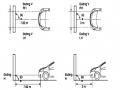
(t) or the vane opening a 0 (t) (Figure 14-6).
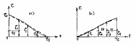
Figure 14-6. Relative opening and closing mode of water direction flap.
2
a. Determine the relative water pressure at the end of the first phase (n = 1) 1 A :
Write the equation for forward wave propagation from A to B (equation 14-3):
B A2 ( v Bv A)
(*)
2 2
Based on the boundary conditions at BB we have
B 0
and the boundary condition at AA we have
v A 2
; Based on the initial condition at B we have
v B v A 0
0 ,
1 A
2
1 A
2
2 0
1 A
0
2
So replace them in (*) we have: A
2 ( 0
2
) and use the symbol at the end
Phase 1: Derive the equation to determine the relative water pressure solution at the end of the first phase:
1 1
1 0
1
2
(14-16)
4
b. Determine the relative water pressure at the end of phase n.
3
4
- Find the water pressure at the end of the second phase (n = 2)
2 A : we write the equation
Forward wave from A to B we have:
THREE
1 A
4
v
3
3 4
2 ( v B
v A
) , based on boundary conditions at B
and A we have:
B 0 and
A 4
. Need to find more
B write equation
3
v
4
Transmitting the wave back from B to A we have:
AB
1 A
2
3
2 3
2 ( v A
v B
) . With
B 0 and
2
3
3
2
Boundary condition at A has: v A
2
, substitute and extract v B
we have solution:
1 2
2 1
(14-17)
2 0 2
- In a similar way, determine the solution for phases 3, 4, ... We have
2n
general solution formula for the end of nth phase ( n A
) any:
1 n
n 1n 1
n 0 2
i i 1
(14-18)
c. Water enters the primary phase and the limiting phase
In calculating and installing pressure pipes, the issue people are concerned with is determining
determine the maximum positive water pressure value to calculate the pipe strength and value
Minimum negative water pressure to check pipe placement to avoid vacuum in
So here we look at this practical issue.
Through actual calculation and operation of the pressure pipeline of the power plant, it is seen that the maximum water pressure max falls into one of two cases: falls at the end of the first phase, that is, max 1 (figure 14-7,a) or falls into the final phase, called the limiting phase, i.e.
max m
(Figure 14-7,b). Next we will determine the water values and these two phases.
Water and first phase max 1
When opening and closing the valve or the flow deflector, the water pressure reaches its maximum value at the end of the first phase, the following phases have smaller values. Therefore, we only need to calculate the water pressure value at the end of this phase. From the solution equation at the end of the first phase (14-16) square 2
and solve we have the solution:
2 ⎡( 02 )
⎤(*)
( 02 ) 2( 22 )
1
0 1
1 ⎢ ⎣1 ⎥ ⎦
Need to choose the sign of the root of (*). If you choose the root with the (+) sign in (*) then if
turbine closing from initial relative opening
0 1 (full load) to fully closed ( 1 0 ) then
2 2 c V max H max
This is absurd. So the solution would be:
1 0 g H 0 H 0
( 02 ) 2( 22 )
1
0 1
2 ⎡ ( 0 2 )
max
⎤(14-19)
1 ⎢ ⎣1 ⎥ ⎦
The first phase of water collision usually occurs in high water column (usually H 150 - 250 m).
Figure 14-7. Diagram of water entering the first phase and the limiting phase.
Water and phase limit max m
During the turbine opening and closing process, the water pressure increases gradually and reaches its maximum value.
into the final phase
max (figure 14-7,b), that is
max m , called water and the limiting phase. To
To establish the formula for calculating water pressure and limiting phase, we use the solution (14-18) written for phase (m-1) and phase m as follows:
1 m 1
m 1
1m 2
m 1
0
2
i i 1
(*)
1 m
m 1m 1
m 0
2
i i 1
(**)
From figure (14-7,b) we can see that
m 1 m
and take the corresponding sides of (*) and (**)
Subtracting each other we have:
( m m 1 )
1
1 m
m
. Consider the opening and closing process according to the rules.
linear law then relative aperture difference
m 1
m
tf
1 m
T s
2 L
c T s
from here
out
1 m m =
m (***).
Here .
2L c Q max LV max is the characteristic coefficient of inertia of the line
c T s 2gF H 0 g H 0 T s
pipe. Solving equation (***) we get water pressure and limit:
(
m 2
2 4 )
(14-20)
In the above formula, the (+) sign corresponds to closing, the (-) sign corresponds to opening the turbine. Water entering the limiting phase often occurs in low-head turbines.
Water phase prediction
1
To determine the maximum water pressure, we use the two formulas (14-19) and (14-20) to calculate, then take the larger value of the two formulas. However, to reduce the calculation volume, we can establish an approximate formula for the two phases above and then compare them to find the standard for judging which phase the water falls into, then use the appropriate formula to calculate.
When calculating approximately consider
1 according to the Taylor expansion, so
2
The formula for the final phase of the first phase (14-16) is:
1 1
1
(1 1 )
1
1
(
1 )
1
0 2 1
2 . 2
2 0 2
2
2 1
0 1
(14-21)
1 1 1
( 0 ) 1
1 0
Similarly approximately for water and the limiting phase we have:
m
2
2
(14-22)
- The condition for water impact is the first phase when:
- The condition for water impact is the limiting phase when:
1 > m
1 < m
or 0 1 ; or 0 1 .
So to determine the maximum water pressure, we first use the above formulas to predict the phase. If it falls into the first phase, use formula (14-19) to calculate. If it falls into the limiting phase, use formula (14-20) to calculate.
Note that: the above calculation formulas are suitable for impulse turbines, however, for counter-attack turbines, the complex opening and closing rules between opening and flow do not follow a linear rule. Therefore, the above calculation is only approximate, for correct calculation, please refer to the calculation by graphical method. In the analytical method, Russian scientist GI Kriptrenko added to formulas (14-21) and (14-22) correction factors to refer to the opening and closing rules of counter-attack turbines as follows:
1
2
1 2b( 0)
(14-21')
m
2
2 b
(14-22')
In which, the correction factor b is taken as follows:
. In case of turbine closure: b = 0.7 - ( n S /1000);
.In case of turbine opening: b + 1.1 - (n S /600).
3. Calculation of water impact in complex pipes
In the above section we have considered the method of calculating water pressure in pipes.
simple, where the characteristics of the water are c,
,
unchanged in length
Pipes and pipes without branches, in practice, when the length of the pipeline is long and the water column is high, it is necessary to change the diameter, wall thickness, even the material of the pipe and the end of the pipe is branched into the generators... for economic purposes. Complex pipes are pipes with water characteristics and sizes that change according to each pipe section. In practice, there are often two common types of complex pipes:
- Pipe diameter decreases from top to bottom, no branches;
- The pipe has a diameter that decreases from top to bottom and has branches.
The exact calculation of this type of pipe is very complicated. The analytical method often leads to an equivalent simple pipe with average characteristics c, V, , , ... and still relies on single pipe formulas for approximate calculations.
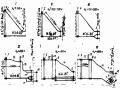
Figure 14-8. Diagram of calculating water impact on complex pipes and drawing a diagram of water pressure impact along the pipe.
* Case 1: pipe with thickness , diameter D and pipe material changes along the pipe length, no branches (figure 14-8,a) with n pipe segments as shown. We get an equivalent simple pipe with the following characteristics:
n
V i max . L i
n
L i
c V
n
L i . V max
n
2 L i
V max i 1; c i 1; max;i 1; t f i 1
n
L i
n Li
2g H 0
g H 0 T sc
i 1
i 1 c i
With the above average characteristics, replacing the formulas of the single pipe, we will calculate the water pressure of the complex pipe that needs to be found.
* Case 2: pipe with branch (figure 14-8,a'):
To calculate the water pressure in a branched pipe to a non-branched pipe with changing characteristics, keep the main pipe sections intact and cut off the dead branch pipe section, replace the parallel branches with a single pipe section. Join the branch pipe sections on the basis of preserving the length and total area of the branch pipe, preserving the wave propagation speed c on the branches. In the above example (Figure 14-8,a'), it is necessary to determine the water pressure when changing the opening of turbines 1 and 2 when turbine 3 is completely closed (branch pipe 3 is a dead branch), then the calculation diagram is converted to case 1, but here the equivalent branch pipe section has length L 1 and area 2F 1 , wave propagation speed c = c 1 (with two branches being the same). Then we calculate as presented in case 1.
4. Draw a graph of water pressure along the pipeline.
The purpose of drawing the maximum water pressure (+) diagram is to determine the water pressure (including static water column plus water pressure) at the pipe cross-sections. Therefore, the water level in the lake or pressure tank must be taken as MNDBT and not subtract the water column loss (Figure 14-8,b).
The purpose of drawing the negative water pressure diagram is to check whether this diagram touches the pipe (ie there is a vacuum in the pipe). If it does, it is best to lower the height of the pipe below the diagram or treat it with a hard belt to ensure the stability of the pipe wall. Therefore, the water level of the lake or the water level in the pressure tank takes MNC and subtracts the water column loss (Figure 14-8,b).
To draw a graph of water pressure along the pipe, we spread the pipe along its length. At the end section of the pipe (AA), we calculate the positive water pressure value H A and water collide with sound H A , and at the cross-section BB near the lake H B0 . Assume that the water pressure along the pipe is distributed according to the rule
straight line, we connect the two ends to get the water pressure distribution chart along the pipe. With the pressure values at the positions placed on the cross-sections CC, AA, BB, we get the water pressure chart along the pipe (figure 14-8,b). In case there is a pressure chamber, we do the same and show the water pressure chart as (figure 14-8, ).
Note that in reality the distribution of water pressure along the pipe depends on the characteristics of the pipe and the initial opening of the CCHD or needle valve, so in reality it is approximate to consider the pressure distribution as a straight line. In fact, if the water state is the first phase, the law of water pressure distribution along the pipe is a concave curve, but in the limiting phase state, it is close to a straight line, as shown in the dashed curve above (Figure 14-8, ).
XIV. 2. 3. Calculation of water impact by graphical method
As seen above, the analytical method is only suitable for impulse turbines but not fully suitable for counter-attack turbines, because in counter-attack turbines, the flow through the turbine during the transition process is very complicated, it depends on many factors such as
aperture characteristic
a 0 of the guide vane, depending on the rotation, on the internal rotation angle
turbine blades ..etc. These factors cannot be expressed mathematically but
main synthetic characteristic curve - built on experimental basis. In addition, using the method