In the current conditions, the use of ABC analysis techniques is carried out through computerized automated inventory management systems. However, in some enterprises that do not have the conditions to automate inventory management, ABC analysis is carried out manually, although it takes more time, it will bring certain benefits.
In addition to relying on the annual value of reserves for grouping, other criteria are also considered such as:
- Changes in forecasting techniques;
- Supply issues;
- Quality of stock;
Maybe you are interested!
-

 Quality Management Step by Step in the Aviation Service Supply Process:
 -
 Car body electrical practice - 8
zt2i3t4l5ee
zt2a3gs
zt2a3ge
zc2o3n4t5e6n7ts
If the voltage is out of specification, replace the wire or connector.
If the voltage is within specification, install the front fog light relay and follow step 5.
Step 5 Check the front fog light switch
- Remove the D4 connector of the fog light switch
- Use a multimeter to measure the resistance of the front fog light switch.
Measurement location
Condition
Standard
D4-3 (BFG) -D4-4 (LFG)
Light switchFront Fog OFF
>10kΩ
D4-3 (BFG) -D4-4 (LFG)
Front fog light switchON
<1 Ω
- Standard resistor
D4 connector is located on the combination switch assembly.
If the resistance is out of specification, replace the combination switch (the fog light switch is located in the combination switch).
If the resistance is within specification, follow step 6.
Step 6 Check wiring and connectors (front fog light relay-light selector switch)
- Disconnect connector D4 of the combination switch assembly
- Use a voltmeter to measure the voltage value of jack D4 on the wire side.
Measurement location
Control modecontrol
Standard
D4-3 (BFG) - (-) AQ
TAIL
11 to 14 V
D4 connector for the wiring of the combination switch assembly
If the voltage does not meet the standard, replace the wire or connector.
If the voltage is within standard, there may have been an error in the previous measurements.
Step 7 Check the front fog lights
- Remove the front fog light electrical connector.
- Supply battery voltage to the fog lamp terminals
Jack 8, B9 of front fog lamp on the electrical side
blind first.
Power supply location
Terms and Conditions
Battery positive terminal - Terminal 2Battery negative terminal - Terminal 1
Fog lightsbefore morning
- If the light does not come on, replace the bulb.
If the light is on, re-plug the jack and continue to step 8.
Step 8 Check wiring and connectors (relay and front fog lights)
- Disconnect the B8 and B9 connectors of the front fog lights.
- Use a voltmeter to measure voltage at the following locations:
Measurement location
Switch location
Terms and Conditions
B8-2 - (-) AQ
Electric lock ON TAIL size switchFog switch ON
11 to 14 V
B9-2 - (-) AQ
Electric lock ONTAIL size switch Fog switch ON
11 to 14 V
B8 and B9 connectors on the front fog lamp wiring side
Voltage is not up to standard, repair or replace the jack. If up to standard, there may have been an error in the measurement process.
2.2.4. Procedure for removing, installing and adjusting fog lights 1. Procedure for removing
- Remove the front inner ear pads
Use a screwdriver to remove the 3 screws and remove the front part of the front inner ear liner
-Remove the fog light assembly
+ Disconnect the connector.
+ Use a screwdriver to remove 3 screws to remove the fog light cover
2. Installation sequence
-Rotate the fog lamp bulb in the direction indicated by the arrow as shown in the figure and remove the fog lamp from the fog lamp assembly.
-Rotate the fog light bulb in the direction indicated by the arrow as shown in the figure and install the light into the fog light assembly.
- Use a screwdriver to install the fog light cover
-Install the electrical connector
Attention: Be careful not to damage the plastic thread on the lamp assembly.
- Install the front inner ear pads
Use a screwdriver to install the front inner bumper with 3 screws.
3. Prepare the vehicle to adjust the fog light convergence. Prepare the vehicle:
- Make sure there is no damage or deformation to the vehicle body around the fog lights.
- Add fuel to the fuel tank
- Add oil to standard level.
- Add engine coolant to standard level.
- Inflate the tire to standard pressure.
- Place spare tire, tools and jack in original design position
- Do not leave any load in the luggage compartment.
- Let a person weighing about 75 kg sit in the driver's seat.
4. Prepare to check the fog light convergence
a/ Prepare the vehicle status as follows:
- Place the car in a dark enough place to see the lines. The lines are the dividing line, below which the light from the fog lights can be seen but above which it cannot.
- Place the car perpendicular to the wall.
- Keep a distance of 7.62 m between the center of the fog lamp and the wall.
- Park the car on level ground.
- Press the car down a few times to stabilize the suspension.
Note: A distance of approximately 7.62 m is required between the vehicle (fog lamp center) and the wall to adjust the convergence correctly. If the distance of 7.62 m cannot be achieved, set the correct distance of 3 m to check and adjust the fog lamp convergence. (Since the target area varies with the distance, please follow the instructions as shown in the figure.)
b/ Prepare a piece of thick white paper about 2 m high and 4 m wide to use as a screen.
c/ Draw a vertical line through the center of the screen (line V).
d/ Set the screen as shown in the picture. Note:
- Keep the screen perpendicular to the ground.
- Align the V line on the screen with the center of the vehicle.
e/Draw the reference lines (H, V LH and V RH lines) on the screen as shown in the figure.HINT:
Mark the center of the fog lamp on the screen. If the center mark cannot be seen on the fog lamp, use the center of the fog lamp or the manufacturer's name mark on the fog lamp as the center mark.
H line (fog light height):
Draw a line across the screen so that it passes through the center mark. Line H should be at the same height as the center mark of the fog light bulb.
Line V LH, V RH (center mark position of left fog lamp LH and right fog lamp RH):
Draw two lines so that they intersect line H at the center marks.
5. Check the fog light convergence
a/ Cover the fog lamp or remove the connector of the other side fog lamp to prevent light from the unchecked fog lamp from affecting the fog lamp convergence test.
b/ Start the engine.
c/ Turn on the fog lights and make sure that the dividing line is outside the standard area as shown in the drawing.
6. Adjust the fog light convergence
Use a screwdriver to adjust the fog light to the standard area by turning the toe adjustment screw.
Note: If the screw is adjusted too far, loosen it and then tighten it again, so that the last rotation of the light adjustment screw is clockwise.
3. Self-study questions
1. Describe the operating principle of the lighting system with automatic headlight function
2. Describe the operating principle of the lighting system with the function of rotating headlights when turning
3. Draw diagram and connect lighting system on Hyundai Porter car
4. Draw diagram and connect lighting system on Honda Accord 1992
5. Draw the lighting circuit on a 1993 Toyota Lexus
LESSON 3 MAINTENANCE AND REPAIR OF SIGNAL SYSTEM
I. IMPLEMENTATION GOAL
After completing this lesson, students will be able to:
- Distinguish between types of signals on cars
- Correctly describe common symptoms and suspected areas causing damage.
- Connecting signal circuits ensures technical requirements
- Disassemble, install, check, maintain and repair the signal system to ensure technical requirements.
- Ensure safety in work and industrial hygiene
II. LESSON CONTENT
1. General description
The signal system equipped on cars aims to create signals to notify other vehicles participating in traffic about the vehicle's operating status such as: stopping, parking, braking, reversing, turning...
Signals are used either by light such as headlamps, brake lights, turn signals….. or by sound such as horns, reverse music….
Just like the lighting system. A signal system circuit usually consists of: battery, fuse, wire, relay, electrical load and control switch. Only some switches of the signal system are on the combination switch. The switches of other signals are usually located in different locations such as in the gearbox or brake pedal……
2. Maintenance and repair
2.1. Turn signals and hazard lights
The installation location of the turn signal is shown in Figure 3.1. The turn signal control switch is located in the combination switch under the steering wheel. Turning this switch to the right or left will make the turn signal turn right or left.
The hazard light switch is used when the vehicle has a problem while participating in traffic. When the hazard light switch is turned on, all the turn signals on the vehicle will light up at a certain frequency. The hazard light switch is usually placed separately from the turn signal switch (some old cars integrate the hazard and turn signal switches on the same combination switch cluster).
Figure 3.1 Turn signal switch Figure 3.2 Hazard switch
The part that generates the flashing frequency for the lights is called a turn signal relay. The turn signal relay usually has 3 terminals: B (positive power supply); E (negative power supply); L (providing the turn signal switch to distribute to the
lamp)
2.1.1. Circuit diagram
To generate the frequency for the turn signal, a turn signal relay is used in the turn signal circuit. The current from the turn signal relay will be sent to the turn signal switch assembly to distribute the current to the turn signal lights for the driver's purpose.
Figure 3.3. Schematic diagram of a turn signal circuit without a hazard switch
1. Battery; 2. Electric lock; 3. Turn signal relay; 4. Turn signal switch; 5. Turn signal lamp; 6. Turn signal lamp; 7. Hazard switch
Figure 3.4 Schematic diagram of turn signal circuit with hazard switch
1. Battery; 2. Combination switch cluster; 3. Turn signal;
4. Turn signal light; 5. Turn signal relay
Today's cars no longer use three-pin turn signal relays (B, L, E) but use eight-pin turn signal relays (figure 3.5) (pin number 8 is used for hazard lights).
For this type, the current supplying the turn signal lights is supplied directly from the turn signal relay to the lights.
div.maincontent .p { color: black; font-family:"Times New Roman", serif; font-style: normal; font-weight: normal; text-decoration: none; font-size: 14pt; margin:0pt; } div.maincontent p { color: black; font-family:"Times New Roman", serif; font-style: normal; font-weight: normal; text-decoration: none; font-size: 14pt; margin:0pt; } div.maincontent .s1 { color: black; font-family:"Times New Roman", serif; font-style: normal; font-weight: normal; text-decoration: none; font-size: 13pt; } div.maincontent .s2 { color: black; font-family:"Times New Roman", serif; font-style: italic; font-weight: normal; text-decoration: none; font-size: 14pt; } div.maincontent .s3 { color: black; font-family:"Times New Roman", serif; font-style: normal; font-weight: normal; text-decoration: none; font-size: 14pt; } div.maincontent .s4 { color: black; font-family:"Times New Roman", serif; font-style: normal; font-weight: normal; text-decoration: none; font-size: 13pt; } div.maincontent .s5 { color: black; font-family:"Times New Roman", serif; font-style: normal; font-weight: normal; text-decoration: none; font-size: 13pt; vertical-align: 1pt; } div.maincontent .s6 { color: black; font-family:"Times New Roman", serif; font-style: normal; font-weight: normal; text-decoration: none; font-size: 11pt; } div.maincontent .s7 { color: black; font-family:"Times New Roman", serif; font-style: normal; font-weight: normal; text-decoration: none; font-size: 14pt; vertical-align: -9pt; } div.maincontent .s8 { color: black; font-family:"Times New Roman", serif; font-style: normal; font-weight: normal; text-decoration: none; font-size: 11pt; } div.maincontent .s9 { color: #008000; font-family:"Times New Roman", serif; font-style: normal; font-weight: normal; text-decoration: none; font-size: 14pt; } div.maincontent .s10 { color: black; font-family:"Times New Roman", serif; font-style: italic; font-weight: normal; te
Car body electrical practice - 8
zt2i3t4l5ee
zt2a3gs
zt2a3ge
zc2o3n4t5e6n7ts
If the voltage is out of specification, replace the wire or connector.
If the voltage is within specification, install the front fog light relay and follow step 5.
Step 5 Check the front fog light switch
- Remove the D4 connector of the fog light switch
- Use a multimeter to measure the resistance of the front fog light switch.
Measurement location
Condition
Standard
D4-3 (BFG) -D4-4 (LFG)
Light switchFront Fog OFF
>10kΩ
D4-3 (BFG) -D4-4 (LFG)
Front fog light switchON
<1 Ω
- Standard resistor
D4 connector is located on the combination switch assembly.
If the resistance is out of specification, replace the combination switch (the fog light switch is located in the combination switch).
If the resistance is within specification, follow step 6.
Step 6 Check wiring and connectors (front fog light relay-light selector switch)
- Disconnect connector D4 of the combination switch assembly
- Use a voltmeter to measure the voltage value of jack D4 on the wire side.
Measurement location
Control modecontrol
Standard
D4-3 (BFG) - (-) AQ
TAIL
11 to 14 V
D4 connector for the wiring of the combination switch assembly
If the voltage does not meet the standard, replace the wire or connector.
If the voltage is within standard, there may have been an error in the previous measurements.
Step 7 Check the front fog lights
- Remove the front fog light electrical connector.
- Supply battery voltage to the fog lamp terminals
Jack 8, B9 of front fog lamp on the electrical side
blind first.
Power supply location
Terms and Conditions
Battery positive terminal - Terminal 2Battery negative terminal - Terminal 1
Fog lightsbefore morning
- If the light does not come on, replace the bulb.
If the light is on, re-plug the jack and continue to step 8.
Step 8 Check wiring and connectors (relay and front fog lights)
- Disconnect the B8 and B9 connectors of the front fog lights.
- Use a voltmeter to measure voltage at the following locations:
Measurement location
Switch location
Terms and Conditions
B8-2 - (-) AQ
Electric lock ON TAIL size switchFog switch ON
11 to 14 V
B9-2 - (-) AQ
Electric lock ONTAIL size switch Fog switch ON
11 to 14 V
B8 and B9 connectors on the front fog lamp wiring side
Voltage is not up to standard, repair or replace the jack. If up to standard, there may have been an error in the measurement process.
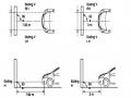
2.2.4. Procedure for removing, installing and adjusting fog lights 1. Procedure for removing
- Remove the front inner ear pads
Use a screwdriver to remove the 3 screws and remove the front part of the front inner ear liner
-Remove the fog light assembly
+ Disconnect the connector.
+ Use a screwdriver to remove 3 screws to remove the fog light cover
2. Installation sequence
-Rotate the fog lamp bulb in the direction indicated by the arrow as shown in the figure and remove the fog lamp from the fog lamp assembly.
-Rotate the fog light bulb in the direction indicated by the arrow as shown in the figure and install the light into the fog light assembly.
- Use a screwdriver to install the fog light cover
-Install the electrical connector
Attention: Be careful not to damage the plastic thread on the lamp assembly.
- Install the front inner ear pads
Use a screwdriver to install the front inner bumper with 3 screws.
3. Prepare the vehicle to adjust the fog light convergence. Prepare the vehicle:
- Make sure there is no damage or deformation to the vehicle body around the fog lights.
- Add fuel to the fuel tank
- Add oil to standard level.
- Add engine coolant to standard level.
- Inflate the tire to standard pressure.
- Place spare tire, tools and jack in original design position
- Do not leave any load in the luggage compartment.
- Let a person weighing about 75 kg sit in the driver's seat.
4. Prepare to check the fog light convergence
a/ Prepare the vehicle status as follows:
- Place the car in a dark enough place to see the lines. The lines are the dividing line, below which the light from the fog lights can be seen but above which it cannot.
- Place the car perpendicular to the wall.
- Keep a distance of 7.62 m between the center of the fog lamp and the wall.
- Park the car on level ground.
- Press the car down a few times to stabilize the suspension.
Note: A distance of approximately 7.62 m is required between the vehicle (fog lamp center) and the wall to adjust the convergence correctly. If the distance of 7.62 m cannot be achieved, set the correct distance of 3 m to check and adjust the fog lamp convergence. (Since the target area varies with the distance, please follow the instructions as shown in the figure.)
b/ Prepare a piece of thick white paper about 2 m high and 4 m wide to use as a screen.
c/ Draw a vertical line through the center of the screen (line V).
d/ Set the screen as shown in the picture. Note:
- Keep the screen perpendicular to the ground.
- Align the V line on the screen with the center of the vehicle.
e/Draw the reference lines (H, V LH and V RH lines) on the screen as shown in the figure.HINT:
Mark the center of the fog lamp on the screen. If the center mark cannot be seen on the fog lamp, use the center of the fog lamp or the manufacturer's name mark on the fog lamp as the center mark.
H line (fog light height):
Draw a line across the screen so that it passes through the center mark. Line H should be at the same height as the center mark of the fog light bulb.
Line V LH, V RH (center mark position of left fog lamp LH and right fog lamp RH):
Draw two lines so that they intersect line H at the center marks.
5. Check the fog light convergence
a/ Cover the fog lamp or remove the connector of the other side fog lamp to prevent light from the unchecked fog lamp from affecting the fog lamp convergence test.
b/ Start the engine.
c/ Turn on the fog lights and make sure that the dividing line is outside the standard area as shown in the drawing.
6. Adjust the fog light convergence
Use a screwdriver to adjust the fog light to the standard area by turning the toe adjustment screw.
Note: If the screw is adjusted too far, loosen it and then tighten it again, so that the last rotation of the light adjustment screw is clockwise.
3. Self-study questions
1. Describe the operating principle of the lighting system with automatic headlight function
2. Describe the operating principle of the lighting system with the function of rotating headlights when turning
3. Draw diagram and connect lighting system on Hyundai Porter car
4. Draw diagram and connect lighting system on Honda Accord 1992
5. Draw the lighting circuit on a 1993 Toyota Lexus
LESSON 3 MAINTENANCE AND REPAIR OF SIGNAL SYSTEM
I. IMPLEMENTATION GOAL
After completing this lesson, students will be able to:
- Distinguish between types of signals on cars
- Correctly describe common symptoms and suspected areas causing damage.
- Connecting signal circuits ensures technical requirements
- Disassemble, install, check, maintain and repair the signal system to ensure technical requirements.
- Ensure safety in work and industrial hygiene
II. LESSON CONTENT
1. General description
The signal system equipped on cars aims to create signals to notify other vehicles participating in traffic about the vehicle's operating status such as: stopping, parking, braking, reversing, turning...
Signals are used either by light such as headlamps, brake lights, turn signals….. or by sound such as horns, reverse music….
Just like the lighting system. A signal system circuit usually consists of: battery, fuse, wire, relay, electrical load and control switch. Only some switches of the signal system are on the combination switch. The switches of other signals are usually located in different locations such as in the gearbox or brake pedal……
2. Maintenance and repair
2.1. Turn signals and hazard lights
The installation location of the turn signal is shown in Figure 3.1. The turn signal control switch is located in the combination switch under the steering wheel. Turning this switch to the right or left will make the turn signal turn right or left.
The hazard light switch is used when the vehicle has a problem while participating in traffic. When the hazard light switch is turned on, all the turn signals on the vehicle will light up at a certain frequency. The hazard light switch is usually placed separately from the turn signal switch (some old cars integrate the hazard and turn signal switches on the same combination switch cluster).
Figure 3.1 Turn signal switch Figure 3.2 Hazard switch
The part that generates the flashing frequency for the lights is called a turn signal relay. The turn signal relay usually has 3 terminals: B (positive power supply); E (negative power supply); L (providing the turn signal switch to distribute to the
lamp)
2.1.1. Circuit diagram
To generate the frequency for the turn signal, a turn signal relay is used in the turn signal circuit. The current from the turn signal relay will be sent to the turn signal switch assembly to distribute the current to the turn signal lights for the driver's purpose.
Figure 3.3. Schematic diagram of a turn signal circuit without a hazard switch
1. Battery; 2. Electric lock; 3. Turn signal relay; 4. Turn signal switch; 5. Turn signal lamp; 6. Turn signal lamp; 7. Hazard switch
Figure 3.4 Schematic diagram of turn signal circuit with hazard switch
1. Battery; 2. Combination switch cluster; 3. Turn signal;
4. Turn signal light; 5. Turn signal relay
Today's cars no longer use three-pin turn signal relays (B, L, E) but use eight-pin turn signal relays (figure 3.5) (pin number 8 is used for hazard lights).
For this type, the current supplying the turn signal lights is supplied directly from the turn signal relay to the lights.
div.maincontent .p { color: black; font-family:"Times New Roman", serif; font-style: normal; font-weight: normal; text-decoration: none; font-size: 14pt; margin:0pt; } div.maincontent p { color: black; font-family:"Times New Roman", serif; font-style: normal; font-weight: normal; text-decoration: none; font-size: 14pt; margin:0pt; } div.maincontent .s1 { color: black; font-family:"Times New Roman", serif; font-style: normal; font-weight: normal; text-decoration: none; font-size: 13pt; } div.maincontent .s2 { color: black; font-family:"Times New Roman", serif; font-style: italic; font-weight: normal; text-decoration: none; font-size: 14pt; } div.maincontent .s3 { color: black; font-family:"Times New Roman", serif; font-style: normal; font-weight: normal; text-decoration: none; font-size: 14pt; } div.maincontent .s4 { color: black; font-family:"Times New Roman", serif; font-style: normal; font-weight: normal; text-decoration: none; font-size: 13pt; } div.maincontent .s5 { color: black; font-family:"Times New Roman", serif; font-style: normal; font-weight: normal; text-decoration: none; font-size: 13pt; vertical-align: 1pt; } div.maincontent .s6 { color: black; font-family:"Times New Roman", serif; font-style: normal; font-weight: normal; text-decoration: none; font-size: 11pt; } div.maincontent .s7 { color: black; font-family:"Times New Roman", serif; font-style: normal; font-weight: normal; text-decoration: none; font-size: 14pt; vertical-align: -9pt; } div.maincontent .s8 { color: black; font-family:"Times New Roman", serif; font-style: normal; font-weight: normal; text-decoration: none; font-size: 11pt; } div.maincontent .s9 { color: #008000; font-family:"Times New Roman", serif; font-style: normal; font-weight: normal; text-decoration: none; font-size: 14pt; } div.maincontent .s10 { color: black; font-family:"Times New Roman", serif; font-style: italic; font-weight: normal; te -
 Effect of Initial Glyphosate Concentration on Processability of Electrochemical Fenton Process
 -
 Cultivation and Production Process of Special Rare Weasel Coffee
 -
 Complete the retail process of kitchen utensils at Website Hanoi.Golmart.vn - 9
- Prices of stock items...
These standards may change the location of stocks. The classification of stocks is the basis for establishing separate control policies for each type of stock.
In inventory management, ABC analysis has the following effects:
- The capital resources used to purchase group A goods are more needed than group C goods, so there needs to be appropriate investment priority in group A management.
- Group A goods need priority in arrangement, inspection and control of physical items. Establishing accurate reports on group A must be done regularly to ensure safety in production.
- In forecasting reserve demand, we need to apply different forecasting methods for different groups of goods. In which, group A needs to be forecasted more carefully than other groups.
- Thanks to ABC analysis techniques, the level of warehouse staff is constantly increasing, because they regularly perform inspection and control cycles for each group of goods.
8.2. Just-in-time (JIT) inventory
8.2.1. Concept of just-in-time inventory
Stocks in the production and supply system are intended to guard against possible contingencies during the production and distribution process. To ensure optimal efficiency in production and business, businesses around the world, especially Japanese businesses, have applied the Just in Time supply model.
Just-in-time inventory is the minimum amount of inventory needed to keep the production system running normally. With the method of organizing supply and just-in-time inventory, people determine quite accurately the quantity of each type of inventory at each time to ensure that goods are delivered to the place of demand at the right time, promptly so that the operation of any place is continuous (Not too early and not too late).
To achieve just-in-time inventory, production managers must find ways to reduce variations caused by internal and external factors of the production process.
8.2.2. Causes of delays in the supply process
There are many reasons for delays or untimely delivery of materials and goods, including:
- Causes related to labor, equipment, and supply sources: not meeting requirements, resulting in products that do not meet standards, or the quantity produced is not enough for the shipment to be delivered.
- Incorrect product and technology design.
- Production departments carry out manufacturing before there are technical drawings or detailed designs.
- Not sure about customer requirements.
- Establishing relationships between stages is not tight.
- The supply system does not ensure the correct requirements of the reserve (causing loss, damage)...
All of the above causes cause changes that affect the amount of reserves in the stages of the business production process of the enterprise.
8.2.3. Solutions to reduce reserves in stages
- Reducing initial inventory: Initial inventory represents the link between the production process and the supply source. Effective approaches to reducing initial inventory are to find ways to reduce the supply variability in quantity, quality, and delivery time.
- Reduce the amount of unfinished products on the production line: If the production cycle can be reduced, this amount of inventory will be reduced. To do this, it is necessary to carefully examine the structure of the production cycle.
- Reduce tools and spare parts: This type of reserve serves the need to maintain, preserve and repair machinery and equipment. This need is relatively difficult to determine accurately. Tools and spare parts are reserved to ensure 3 requirements: maintenance, repair, replacement. Only some types of this activity can be calculated accurately, while some types must use forecasting methods.
- Reduce finished product inventory: finished product inventory comes from customer demand at a certain time. Therefore, if we accurately predict customer demand, we will reduce this type of inventory.
In addition, to achieve the right amount of stock, the administrator needs to find ways to reduce incidents, reduce hidden variations inside, this is an extremely important job in production management. The basic problem to achieve the right time requirement
The point of manufacturing is to produce small lots of goods according to predetermined standards. Reducing lot sizes is a fundamental aid in reducing inventory and inventory costs.
When consumption remains constant, average reserves are determined as follows:
In there:
Q=
Q max + Q min
2
(8.1)
𝑄: Average stock; Q max : Maximum stock; Q min : Minimum stock.
One of the solutions to minimize the amount of stock is to only transfer the stock to where there is real demand, not to where there is no demand yet. Such a transportation system is called the Kaban system by the Japanese.
8.3. Reserve models
When studying reserve models, we need to answer two key questions:
- What quantity of goods in each order has the lowest cost?
- When to place order?
To answer the above 2 questions for different cases, we examine the following 5 models in turn:
8.3.1. Economic Order Quantity (EOQ) Model
The EOQ model was proposed and applied in 1915, and is still used by most businesses today. The inventory control technique based on this model is very easy to apply. The important assumptions of the model are:
- Demand must be known in advance and constant;
- Must know in advance the time from placing an order until receiving the goods and that time remains constant;
- The quantity of goods in each order is made in one shipment and is made at a predetermined time;
- Only consider 2 types of costs: storage costs and ordering costs;
- Inventory shortages do not occur at all if orders are filled correctly. With the above assumptions, the diagram representing the EOQ model is shown in Figure 8.2.
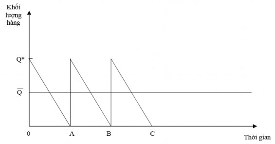
Figure 8.2: EOQ model
In there:
Q* : Quantity of an order (Maximum stock Q max = Q*).
0 : Minimum reserve level (Q min = 0).
Q=Q*
2
∶ is the average reserve.
0A = AB = BC is the time from receipt of goods until the goods of a reserve batch are used up.
With this model, inventories will decrease at a constant rate because demand does not change over time.
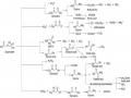
a. Determine the basic parameters of the EOQ model
The objective of most inventory models is to minimize the total inventory cost. With the above assumptions, there are two types of costs that change when inventory levels change. These are the holding cost (C lk ) and the ordering cost (C dh ), while the purchasing cost (C mh ) does not change. The relationship between these costs can be illustrated in Figure 8.3.
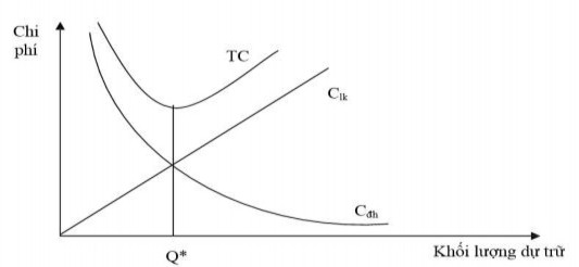
Figure 8.3: Cost types of the EOQ model
In there:
C dh : Order cost curve. C lk : Inventory cost curve. TC : Total inventory cost curve.
Q * : Optimal stock quantity (Optimal order quantity).
From the above model we have:
TC = C dh + C lk (8.2)
DQ
In there:
Or TC = Q x S + 2 x H (8.3)
D : Demand for inventory in a period. Q : Quantity in an order.
S : Cost of placing an order.
H: Cost of storing 1 unit of inventory in 1 period.
We will have the optimal order quantity (Q * ) when the total cost is minimum. To have TC min then TC ' Q = 0.
2
DS H 2DS
We have: TC' = - + => Q =
Q 2 2 H
So Q * = 2DS
H (8.4)
For example: A company specializing in manufacturing cars must use steel plates with a demand of 1000 plates/year. The ordering cost is 100,000 VND/order. The storage cost is 5,000 VND/plate/year. Determine the optimal order quantity?
The optimal order quantity is determined as follows:
Q * = 2DS = 2(1,000)(100,000)
H 5,000 = 200 (sheets)
Thus we can determine the desired orders in a year and the average interval between two orders.
The desired order quantity is determined as follows:
D
Q = =
Q ∗
1000
200 = 5 (orders/year)
The interval between two orders (T) is calculated by the following formula:
Number of working days in a year (N)
T =
Desired order quantity (O đ )
(8.5)
Assuming the company works 300 days a year, the gap between two orders will be:
300
T = 5 = 60 days
Total inventory cost is calculated as follows:
D
TC = x S +
Q ∗
Q ∗
2 x H
In the above example, the total cost of inventory is:
TC =
1,000
200 x 100,000 +
200
2 x 5,000 = 1,000,000 VND
b. Determine the reorder point (ROP)
In the EOQ inventory model, we assume that the receipt of an order is done in one shipment. In other words, we assume that the firm will wait until the inventory is depleted before placing an order and will receive it immediately. However, in reality, the time from placing an order to receiving the goods can be several hours or even as long as months. Therefore, the reorder point (ROP) decision is determined as follows:
Reorder point: ROP = dx L (8.6) Where:
L: Time from order to receipt of goods (Leading time). d: Daily consumer demand for inventory.
D
d =
N
In there:
(8.7)
D: Demand for inventory in a period N: Number of production days in a year
Represent ROP on the following diagram:
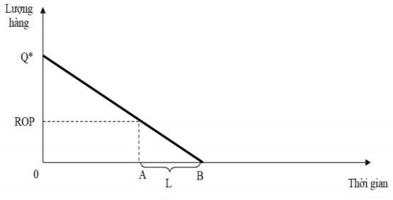
Figure 8.4: ROP model
For example: Dong Tien Electronics Company has a demand for T512 wire of 8,000 units/year. Working time in a year is 200 days. Waiting time for goods is 3 days.
8,000
The reorder point will be: ROP = 200 x 3= 120 units
If the business accepts a safety stock (insurance stock), the reorder point will add this safety stock.
8.3.2. Production Order Quantity (POQ) Model
The production order quantity model is applied in cases where the quantity of goods is delivered continuously, the goods are accumulated gradually until the order quantity is fully assembled. This model is also applied in cases where the enterprise both produces and sells or the enterprise produces its own materials for use. In these cases, it is necessary to pay attention to the daily production level of the manufacturer or the supply level of the supplier.
In the POQ model, the assumptions are basically the same as the EOQ model, the only difference is that the goods are delivered in multiple shipments. Using the same method as the EOQ, the optimal order quantity Q * can be calculated .
If we call:
Q : Order quantity;
P: Production level (Daily supply level); d: Daily demand;
H: Cost of storing 1 unit of inventory for 1 year;
t : Production time to have enough quantity for 1 order (or supply time). The POQ model is shown in Figure 8.5.
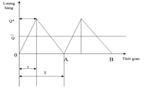
Figure 8.5: POQ model
In this model:
Reserve level
max =
Total number of units supplied (produced) during period t
Total number of units
- used in
time t
(8.8)
That is: Q max = Pt – dt
Q
On the other hand Q = Pt, so: t = P
Substitute the formula for calculating the maximum reserve level into the formula:
Q max
= P Q
- d QQ. (1 - d )
P
P =
Q
So C lk = 2 (1 -
P
d D
) H and C have the following equations : x S
PQ
To find the optimal order quantity Q *, we also apply the same method as in the EOQ model and find:
2DS
*
Q =d
H(1 - P )
(8.9)
For example: Company A specializes in manufacturing spare parts at a rate of 300 units/day. This type of spare part is used 12,500 units/year and the company works 250 days/year. The storage cost is 20,000 VND/unit/year, the cost of ordering each time is 300,000 VND. How much is the production order quantity?
Apply the formula:
In which: d = 12,500 / 250 = 50
P = 300
D = 12,500
S = 300,000
H = 20,000
2DS
*
Q =d
H(1 - P )
2 x 12,500 x 300,000
Instead we have: Q * == 671 units
20,000(1 - 50 )
300
8.3.3. Shortage of stock (BOQ) model
In the above two models of stockpiling, we do not accept that there is a shortage of stock throughout the entire stockpiling process. In reality, there are many cases where the enterprise intends to have a shortage because if it maintains an additional unit of stock, the loss cost is greater than the value gained. The best way in this case is for the enterprise to not stock more goods from the efficiency point of view.