Applied Mechanics

PREFACE

Applied mechanics is a part of basic knowledge for engineers in engineering fields, so this subject is arranged in the training program of many universities such as: Hanoi University of Science and Technology, Transport, Irrigation, Construction, ... At Nam Dinh University of Technical Education, this subject is taught to undergraduate students majoring in Electricity - Electronics. Currently, universities have their own teaching materials for this subject with different names such as Basic Mechanics, Technical Mechanics, etc. with very different content, duration and amount of knowledge due to the characteristics of the industry.

Therefore, it is very necessary to compile a separate Applied Mechanics course for students of Nam Dinh University of Technical Education. According to the Applied Mechanics course program built to teach students of Nam Dinh University of Technical Education, the content of the course includes three parts: Absolute solid mechanics, deformation solid mechanics (Strength of materials) and machine parts, in which the Absolute solid mechanics and machine parts are written in 3 chapters including content on statics, kinematics and dynamics of point materials and mechanical systems. The Deformable solid mechanics part is written in 1 chapter including content on simple and complex forms of force resistance of bars.

The lecture book is written on the basis of the Applied Mechanics course program. The compiler has tried to present the basic issues of Mechanics from a modern perspective, ensuring the pedagogical and quality requirements of a university lecture. The knowledge presented in this lecture is the minimum knowledge, necessary to equip the basic mechanical knowledge in the knowledge system provided to students, especially for non-mechanical students.

This is the first time the textbook has been compiled, so it certainly has many shortcomings. We look forward to receiving comments from colleagues and students to have the conditions to revise and improve the textbook to better serve the teaching and learning work. Comments and contributions should be sent to the address: Department of Basic Engineering, Faculty of Mechanical Engineering, Nam Dinh University of Technical Education.

Editorial team

INDEX

FOREWORD 1

TABLE OF CONTENTS 3

Part 1: ABSOLUTE SOLID MECHANICS 5

Chapter 1 5

DYNAMICS 5

1.1. POINT 5 DYNAMICS

1.1.1. Vector method 5

1.1.2. Cartesian coordinate method 7

1.1.3. Natural coordinate method 9

1.1.4. Some common movements 12

1.2. ABSOLUTE SOLID KINEMATICS 14

1.2.1. Basic movements of solids 14

1.2.2. Parallel motion of solids 22

1.3. COMBINED MOTION OF POINTS AND RIGS 33

1.3.1. Motion combination of point 33

1.3.2. Motion of solid objects 37

1.4. MECHANICAL DYNAMICS 42

1.4.1. Some concepts 42

1.4.2. Flat four-link hinge mechanism 42

1.4.3. Variations of the four-link mechanism 43

1.4.4. Cam mechanism 45

1.4.5. Gear mechanism 46

REVIEW QUESTION 51

Chapter 2 52

STATICS 52

2.1. BASIC CONCEPTS AND LAWS OF STATICS 52

2.1.1. Basic concepts 52

2.1.2. Laws of statics 57

2.1.3. Consequences 61

2.2. SURVEY OF FORCE SYSTEM 64

2.2.1. Plane force system 64

2.2.2. Space force system 74

REVIEW QUESTION 83

Chapter 3 84

DYNAMICS 84

3.1. BASIC LAWS OF DYNAMICS AND DIFFERENTIAL EQUATIONS OF MOTION OF MATERIAL POINTS 84

3.1.1. Concepts 84

3.1.2. Basic laws of dynamics 84

3.1.3. Differential equation of motion of a point particle 86

3.1.4. Two basic problems of dynamics 87

3.2 DYNAMICS OF SYSTEM 89

3.2.1. Concepts 89

3.2.2. Dalambare Principle 93

3.3 GENERAL THEOREMS OF SYSTEM DYNAMICS 96

3.3.1. Momentum theorem and center of mass motion theorem 97

3.3.2. Angular momentum theorem 102

3.3.3. Kinetic energy theorem 106

3.3.4. Theorem of conservation of mechanical energy 114

3.4. DYNAMICS OF SOLIDS 117

3.4.1. Solid objects in translational motion 117

3.4.2. An object rotating around a fixed axis with angular velocity  and angular acceleration  117 3.4.3. A solid object is a flat plate moving in a parallel plane 118

REVIEW QUESTIONS 120

Part 2: MECHANICS OF DEFORMED SOLIDS 121

Chapter 4 121

MECHANICS OF DEFORMABLE SOLIDS 121

4.1. INTRODUCTION 121

4.1.1. Concepts of bar 121

4.1.2. Internal force - Stress 122

4.1.3. Variable cross-section method - internal force components on cross-section

................................................................ ................................................................ ..........................123

4.1.4. Relationship between stress and internal force components on cross section 124

4.1.5. Deformation 125

4.1.6. Basic assumptions about materials 126

4.2. TRUE STRETCHING-COMPRESSION 127

4.2.1. Concept 127

4.2.2. Internal forces and internal force diagrams 127

4.2.3. Stress on cross section 128

4.2.4. Intensity conditions - three basic problems 134

4.3. PURE TORSION OF STRAIGHT BARS 135

4.3.1. Concept 135

4.3.2. Cradle

force

and cradle chart

force

................................................................ ..........................136

4.3.3. Stress on cross section 137

4.3.4. Intensity conditions – three basic problems 141

4.4. FLAT BENDING OF STRAIGHT BARS 143

4.4.1. Concept 143

4.4.2. Internal forces and internal force diagrams 143

4.4.3. Stress on cross section 146

4.4.4. Intensity conditions - three basic problems 154

4.5. COMPLEX BEARING BARS 156

4.5.1. Oblique bending bar 158

4.5.2. Simultaneous bending and tension (compression) 161

4.5.3. Eccentric tension (compression) 165

4.5.4. Simultaneous twisting and bending 167

4.5.5. General bearing bars 171

REVIEW QUESTION 172

REFERENCES 173

Part 1: ABSOLUTE SOLID MECHANICS

Chapter 1 KINEMATICS

1.1. POINT DYNAMICS

In the kinematics of a point, we study the motion of a point with respect to a chosen reference system. For a clear and concise description of the characteristics of the motion, we use the vector method. For convenient calculations, we use coordinate methods such as the Cartesian coordinate method, the natural coordinate method, and the vector method.

1.1.1. Vector method

1.1.1.1. Equation of motion

Consider point M moving in the Oxyz reference system (Figure 1.1). The position of point M is determined by



vector r OM . Point M moves, therefore



r changes over time:



r r ( t ) (1.1)

Equation (1.1) is called the vector equation of motion of point M.

Note that point M moves continuously, at each moment, point M occupies a specific position and has a specific direction of movement.



Figure 1.1

Therefore r ( t ) is a continuous, single-valued function.

The set of positions of a point in the reference space is called its trajectory in that reference frame. Equation (1.1) is the parametric equation of the trajectory. If the trajectory is a straight line, then the motion is called rectilinear motion. If the trajectory is a curve, then the motion is called curvilinear motion. And then, people often use the name of the trajectory curve to name the motion.

1.1.1.2. Speed of movement

One of the basic characteristics of the motion of a point is the concept of velocity with respect to a chosen frame of reference. We will rigorously formulate the concept



this concept. Suppose at time t, the point is at position M determined by r OM . At the time



else t 1 = t + ∆t, the point at position M 1 is determined by

r 1 OM 1

(Figure 1.2). As follows

time interval ∆t the point moves a distance:



MM 1 r 1 r r

Figure 1.3

Figure 1.2

The velocity of a point at time t is determined as follows:



   r



dr 

v  lim v tb  lim

 t  0

 t dt r

(1.2)

 t  0

Thus, the velocity of a point is the first derivative with respect to time of the position vector.



of that point. The velocity vector v is directed tangentially to the trajectory at point M toward

movement. The unit of speed is meter/second, symbol m/s.

1.1.1.3. Motion acceleration

Suppose at time t, the point at position M has a velocity of



v . At time t 1 = t +

∆t, the point at position M 1 has a velocity of

v 1 . Thus, after time interval ∆t, the velocity of



variation point of a quantity

v v 1 v .



Quantity

a tb   v /  t

is called the average acceleration of the point in the interval

time ∆t, from time t. Vector



a tb

direction along the vector



 v (Figure 1.3).

The acceleration of a point at time t is determined as follows:



 v



dvd 2r 

a  lim a tb

 t  0

 lim  t dt

 t  0

r

dt2

(1.3)

Thus, the acceleration of a point is the first derivative with respect to time of the velocity vector and is equal to the second derivative with respect to time of the position vector of that point. The unit of acceleration is: meter/second 2 , symbolized as m/s 2 .

1.1.1.4. Comments on some properties of motion

First of all, we present a standard for commenting on straight and angular motion.



curvilinear motion of a point. When a point moves in a straight line, the velocity vector v always remains constant.



vector method

v and vector a always have the same direction. Therefore, vector v a 0 .

Conversely, when the moving point is curved, the vector



v generally changes both in direction and

as numerical values. The standard vectors observe:



v and vector



a are generally not in the same direction. Therefore we have the criterion



    0 : Motion in parallel

v a 

   0: Curve motion

Now we give the criteria for judging the uniformity and variability of motion. Motion is uniform when the value of velocity v remains constant. Motion speeds up or slows down depending on whether the value of velocity increases or decreases over time.

Note that the change in v 2 represents the change in the value v of the velocity. We have:

d ( v 2 )  d ( v 2 ) 

service

2 v .



 2 and

dt dt

From there, we draw the following criteria:



  0 : Uniform motion

and 

   0 : Motion of the variable



In the second case, if the motion slows down.

1.1.2. Cartesian coordinate method

1.1.2.1. Equation of motion

v a

> 0 then the motion is getting faster

v a

< 0 is

The position of point M is determined by the three coordinates x, y, z of the point in the Cartesian coordinate system perpendicular to Oxy (Figure 1.4)



r x . i yj zk

When point M moves, x, y, z change continuously over time. So the equations of motion have the form:

x=x(t); y = y(t); z = z(t) (1.4)

1.1.2.2. Movement speed

According to formula (1-2) we have:



Figure 1.4

v  dr  d





dx  dy  dz 

dt dt

( xiyjzk )

ijk

dt dt

Projecting the equality onto the three coordinate axes, we get:

v dx 

dy 

dz 

(1.5)

x dt

x ; v y

dt y ; v z dt z ;

Based on the expressions (1.5), we can easily determine the magnitude and the cosines of



direction of velocity v :

v 2 v 2 v 2

xyz



v v 

and x



x 2 y 2 z 2

y

vs.

cos( Ox , v ) 

;cos( Oy , v ) 

;cos( Oz , v ) 

etc.

1.1.2.3. Motion acceleration

Similar to determining the velocity component expressions, from formula (1.3) we have:



DVD 

d 

a  ( vi v

xy dt

j  v z k )  dt  xi  yj  zk 



dv x 



service 



dv z 











= i 

j k  xi  yj  zk 

dt dt

dt 

From there we get the projection of acceleration a on the coordinate axes:

a dv x

x dt



 x ;

v y 

medical service



 y ;

v z 

dv z dt



 z ;

(1.6)

From (1.6) we can also easily determine the magnitude and direction cosines of a :

a 2 a 2 a 2

xyz



x 2 y 2 z 2



a a 



cos( Ox , a ) 



x ; cos( Oy , a ) 

a a

y ; cos( Oz , a )  z

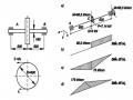
Example 1.1. The motion of point M in the Oxy plane is determined by the equation:

x b sin  t ; y d cos  t (1.7)

In which: b, d, ω, are positive constants. Determine the trajectory equation, magnitude of velocity, acceleration of point M at time t 1 = π/2ω. Then determine the equation of the endpoint of the velocity vector.

Solution:

To find the trajectory equation, we just need to find a way to eliminate the time parameter t in the equations of motion. In this example, from the equations of motion we deduce:

sin  t  x

cos  t  y

Due to the property sin 2  t  cos 2  t  1, we have the orbit equation:

x 2 y 2 

b 2 d 2 1

So the orbit is an ellipse with semi-axes b and d (Figure 1.5). From equation (1.7) we calculate the derivatives with respect to t:



v x x b cos  t , v yy  d sin  t



a x  b 2 sin  t ;



a y  d 2 cos  t

M 0

a 1

M 1

v 1

M 0 '

v 1

M 1 '

a) b)

Figure 1.5

At time t = π/2ω, point M is at position M 1 (x 1 = b; y 1 = 0) and its velocity and acceleration projections have the form:

v 1 x a 1 x

 0

 b 2

v 1 y

a 1 y

 -d 

 0

To draw the velocity vector endpoint (also called the velocity initial line), we choose on

The velocity plane of the perpendicular axis system 0 1 x 1 y 1 is as follows (Figure 1.5)

x 1  v x   b cos  t ; y 1  v y   d sin  t

Eliminating t from the parametric equations of the velocity vector endpoints, we get the equation:

11 1

b 2 2d 2 2

(1.8)

Maybe you are interested!

This is the equation of the velocity vector endpoint in coordinate form. In figure 1.5, the points M' 0 , M', M' 1 on the velocity vector endpoint correspond to the points M 0 , M, M 1 on the orbit.

1.1.3. Natural coordinate method

1.1.3.1. Equation of motion

The natural coordinate method is applied when the trajectory of the point is known in advance. Suppose the trajectory (C) of the point is in a spatial reference system. Choose an arbitrary point O on the trajectory as the origin and

OM (C)

Figure 1.6

determine the positive direction on the orbit (Figure 1.6). The position of point M is determined by the degree

algebraic length of arc OM s

Point M moves so s changes with time. Equation: