Quality Evaluation Criteria of ECG Signal Recognition Model

Table 4.1. Distribution of the number of training samples and test samples of 7 types of arrhythmias from the MIT-BIH database

Rhythm type

Table 4.2. Table dividing the number of study samples and test samples of the 2 types of rhythms

Rhythm type

In Table 4.1 is the number of heart rate types used in the learning and testing of the recognition model. The limited number of heart rate types (e.g. E, I beats) is due to the limitation in the MIT-BIH database [15]. The original number of normal heart rates N is very high, but we consider these as simple beats for classification and to make the final results generally more independent of the number of samples in each group, the author limits the number of heart rates used in the experiments to a reasonable level usually around 1000 beats.

To generate the feature vector and corresponding output signal from the ECG signal records in the MIT-BIH database, we follow the following procedure:

- QRS complex separation: Because in the MIT-BIH database, ECG signals have been marked with R peak positions and have been labeled with disease classification by specialized doctors, so for each QRS complex sample, in this case, there is no need to use the R peak determination algorithm as presented in section 2.2, but only need to sequentially read the R peak positions of the QRS complex in the ECG signal line, separate the QRS complex by cutting a 250ms window around the R peak (125ms before and 125ms after the R peak position).

1

- Expand the QRS complex extracted above according to the Hermite polynomials according to formula 4.1 to determine the first 16 expansion coefficients as characteristics.



n ( x )  

 2 n n !  2e

x 2

2 H n ( x )

(4.1)

- Determine the RR distance from the considered R peak to the previous R peak to make the 17th feature. The average value of the last 10 RR segments will be the 18th feature of the considered QRS complex.

Thus, each QRS complex is separated into 18 characteristics, the output is the code of the disease type of the rhythm under consideration (already marked in the MIT-BIH database ), for example with 7 different rhythm types the corresponding output will be 7 channels with values ​​0 and 1 (6 channels are 0 and the channel with the code corresponding to the disease type will have value 1).

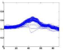
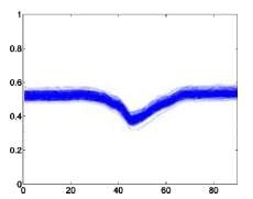
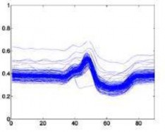
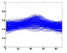
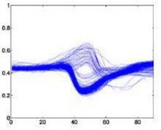
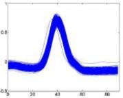
The following is a superimposed image of the samples of 6 types of disease rhythms with the number as shown in Table 4.1. From Figure 4.1, it can be seen that the major obstacle in recognizing ECG signals is the huge variation in amplitude and shape of heart beats belonging to the same disease type [23]. Moreover, some types of rhythms belonging to different diseases can also be similar in morphology . Therefore, we can see that the problem of classifying ECG signals is a difficult problem.

Atrial premature beats – A Ventricular premature beats – E

Left bundle branch block –L Right bundle branch block –R

Ventricular Fibrillation – I Ventricular Premature Contractions – V

Figure 4.1. QRS complex patterns of rhythms A, E, L, R, I and V

4.1.2. MGH/MF Database

In addition, the thesis also uses the second database set, MGH/MF [35, 36], this database set includes 250 records of ECG signals, collected from 250 cardiovascular patients in intensive care rooms, operating rooms, cardiac catheterization laboratories, etc. at Massachusetts General Hospital. The thesis chooses to use ECG signal samples of 20 records with code numbers: 029, 030, 058, 105, 106, 107, 108, 110, 111, 114, 117,

119, 121, 123, 124, 125, 128, 131, 137, 142, taking out a total of 4500 samples with 3 types of rhythm: Normal (N -Normal sinus rhythm), premature ventricular contraction (V-Premature ventricular contraction) and supraventricular premature beat (S-Supraventricular premature beat). The detailed number of samples used is listed in Table 4.3 and Table 4.4 below:

Table 4.3. Table of division of number of study samples and test samples of 3 types of rhythms

Rhythm type

Table 4.4. Table dividing the number of study samples and test samples of the 2 types of rhythms

Rhythm type

Ventricular extrasystole – V Supraventricular arrhythmia – S Normal – N

Figure 4.2. QRS complex pattern of V, S, N rhythms

To generate the feature vectors and corresponding output signals from the ECG signal records in the MGH/MF database, we proceed similarly to the MIT-BIH database.

4.2. Criteria for evaluating the quality of the ECG signal recognition model

The recognition models (single and combined models) are evaluated using the following criteria:

- Number of incorrectly identified samples;

- FN ( False Negative ): Number of false negative diagnoses, that is, cases where the patient has the disease but is misdiagnosed as normal;

- TN (True Negative ): Number of correct negative diagnoses;

- FP (False Positive): Number of false positive diagnoses, meaning cases where the patient is normal but diagnosed with the disease;

- TP (True Positive ): Number of cases with correct positive diagnosis;

- Sensitivity (True Positive Rate) : The rate of correct positive diagnosis,

Sensitivity 

TP TP  FN

.100%

(4.2)

- Specificity (True Negative Rate): Rate of correct negative diagnosis

Specificity 

TN TN  FP

.100%

(4.3)

The recognition model has high quality and reliability when:

- Number of falsely identified samples, number of false positive diagnoses FP, number of false negative diagnoses FN low;

- Correct positive diagnosis rate Sensitivity , correct negative diagnosis rate

The higher the specificity ;