Illustration of Convergence Point Cx in Photographs and in 3D

- Evaluation of tendon healing on MRI based on Sugaya's classification113,114 :

+ Grade I: Suitable rib thickness, uniform rib.

+ Grade II: Appropriate tendon thickness, high signal at a part inside the tendon.

+ Grade III: The tendon is thinner than normal but not continuously lost.

+ Grade IV: Discontinuity of tendon more than one slice, signs of small tears.

+ Grade V: Continuous loss of tendon in multiple slices indicates moderate or large tear.

- Ultrasound evaluation of tendon healing based on Sugaya's classification113,114 :

+ Type I: CX tendon after suturing has sufficient thickness (> 2mm) with normal echogenic structure such as hyperechoic tendon and fiber structure on slices

+ Type II: CX tendon after suturing has sufficient thickness (> 2mm) with partial hypoechoic.

+ Type III: CX tendon after suturing has insufficient thickness (< 2mm), no discontinuity

+ Type IV: There is a small discontinuity, full thickness, good tendon edges, suggesting a small tendon tear.

+ Type V: There is a large discontinuity, the inner edge is not observed below the MCV arch, suggesting a moderate or large tear.

2.4.5. Data analysis and processing

Clean all data before entering data. Enter data using Epidata 3.1 software and process data using STATA 15.0 software.

 Medical statistical algorithms used:

- Descriptive statistics: qualitative variables (number; percentage %); quantitative variables (mean, SD, min-max), if data is not normally distributed (mean, SD, median, min-max).

- Statistical analysis: compare the differences between

 Quantitative variables:

- Compare 2 groups: If the data is normally distributed, use the parametric T-test (independent t-test; paired t-test). Use non-parametric test when the data is normally distributed.

non-standardized (independent comparison: Mann-whitney test; paired comparison: Wilcoxon paired t-test).

- Compare >2 groups: If the data are normally distributed and the variance is homogeneous, use the ANOVA statistical test. In case the data are normally distributed but the variance is not homogeneous or the data is not normally distributed, use the Krusal-wallis test for >2 groups.

 Qualitative variables: Use Chi-square statistical test, Fisher-exact test correction when more than 25% of cells have expected value < 5.

Data are presented in tables and illustrative charts.

2.5. ETHICAL ASPECT

- Dissection specimens must be authorized by the preservation department, on a recognized legal basis.

- Patients are thoroughly explained and provided with full information about their illness, surgical methods and voluntarily participate in the research.

- Respect and confidentiality of personal information.

- Research complies with ethical regulations in biomedical research.

- The topic has been approved by the Medical Ethics Council of Hanoi University of Medicine and Pharmacy.

CHAPTER 3

RESEARCH RESULTS

3.1. RESULTS OF ANATOMY RESEARCH

Through the process of dissecting and studying 20 shoulder joint samples of 10 fresh cadavers, including 4 females and 6 males with an average age of 63.2, we obtained the following data:

3.1.1. Characteristics of the rotator cuff tendon attachment to the greater tuberosity

- Going along the border of the supraspinatus, infraspinatus, and rotator cuff muscles towards the attachment point, we see that they tend to converge at a point located on the raised area on the outer edge of the greater tubercle of the humerus. We temporarily call this the "CX convergence point" (T point) and this raised area is called the "CX convergence area".

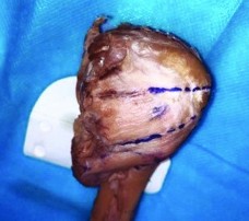
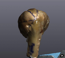
Figure 3.1. Illustration of CX convergence point on photo and in 3D

* Source: Research autopsy photos

- The tendons of the supraspinatus, infraspinatus and teres minor muscles intertwine with each other near the attachment to the greater tubercle.

- According to the dissection along the border of the CX muscles mentioned above, we see that the attachment area of ​​the supraspinatus tendon infraspinatus has a trapezoidal shape, the area

The teres minor tendon has a triangular shape. The supraspinatus, infraspinatus, and teres minor tendons attach to the upper, middle, and lower parts of the greater tubercle of the humerus, respectively.

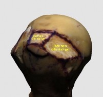
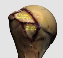
Figure 3.2. Image of supraspinatus, infraspinatus, and small round tendon attachment areas

* Source: Research autopsy photos

- According to the stages of the suturing technique used in the study, the outer edge of the CX tendon attachment is the most ideal position to anchor the CX tendon suture to help restore the torn tendon according to the correct anatomy. Draw landmarks on the 3D file of the scanned specimen and measure the indexes of the outer edge of the CX tendon attachment for application during surgery.

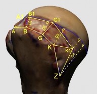
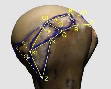
Figure 3.3. Illustration of how to measure the landmarks needed to determine the outer edge of the CX tendon attachment area (B, G, K, Z)

* Source: Research autopsy photos

 The anterolateral border of the supraspinatus tendon, this is an important point as a landmark to determine the next positions. This point is determined based on the

Fixed landmarks that can be observed on dissected bodies and applied during surgery are the lateral border of the intertubercular groove, the border of the articular cartilage, and the convergence point:

Table 3.1. Anterolateral border of the supraspinatus tendon

Dimensions (mm)

Average ± SD	Max	Min
KC to the outer edge of the intertubular sulcus (BA)	7.54±0.615	9.42	6.96
KC to the edge of the articular cartilage (D 1 )	10.01± 1.61	14.46	8.03
KC to the convergence point (TB)	7.80±2.02	5.21	12.38

Maybe you are interested!

• Research on treatment of rotator cuff tears using modified Mason-Allen tendon endoscopic suturing technique and creating micro-damage at the attachment area - 2
• Illustration of Point Contact and Line Contact Cables. A, Point Contact Cable; B, Line Contact Cable
• Qos Assurance Methods for Multimedia Communications zt2i3t4l5ee zt2a3gs zt2a3ge zc2o3n4t5e6n7ts low. The EF PHB requires a sufficiently large number of output ports to provide low delay, low loss, and low jitter. EF PHBs can be implemented if the output port's bandwidth is sufficiently large, combined with small buffer sizes and other network resources dedicated to EF packets, to allow the router's service rate for EF packets on an output port to exceed the arrival rate λ of packets at that port. This means that packets with PHB EF are considered with a pre-allocated amount of output bandwidth and a priority that ensures minimum loss, minimum delay and minimum jitter before being put into operation. PHB EF is suitable for channel simulation, leased line simulation, and real-time services such as voice, video without compromising on high loss, delay and jitter values. Figure 2.10 Example of EF installation Figure 2.10 shows an example of an EF PHB implementation. This is a simple priority queue scheduling technique. At the edges of the DS domain, EF packet traffic is prioritized according to the values ​​agreed upon by the SLA. The EF queue in the figure needs to output packets at a rate higher than the packet arrival rate λ. To provide an EF PHB over an end-to-end DS domain, bandwidth at the output ports of the core routers needs to be allocated in advance to ensure the requirement μ > λ. This can be done by a pre-configured provisioning process. In the figure, EF packets are placed in the priority queue (the upper queue). With such a length, the queue can operate with μ > λ. Since EF was primarily used for real-time services such as voice and video, and since real-time services use UDP instead of TCP, RED is generally not suitable for EF queues because applications using UDP will not respond to random packet drop and RED will strip unnecessary packets. 2.2.4.2 Assured Forwarding (AF) PHB PHB AF is defined by RFC 2597. The purpose of PHB AF is to deliver packets reliably and therefore delay and jitter are considered less important than packet loss. PHB AF is suitable for non-real-time services such as applications using TCP. PHB AF first defines four classes: AF1, AF2, AF3, AF4. For each of these AF classes, packets are then classified into three subclasses with three distinct priority levels. Table 2.8 shows the four AF classes and 12 AF subclasses and the DSCP values ​​for the 12 AF subclasses defined by RFC 2597. RFC 2597 also allows for more than three separate priority levels to be added for internal use. However, these separate priority levels will only have internal significance. PHB Class PHB Subclass Package type DSCP AF4 AF41 Short 100010 AF42 Medium 100100 AF43 High 100110 AF3 AF31 Short 011010 AF32 Medium 011100 AF33 High 011110 AF2 AF21 Short 010010 AF22 Medium 010100 AF23 High 010110 AF1 AF11 Short 001010 AF12 Medium 001100 AF13 High 001110 Table 2.8 AF DSCPs The AF PHB ensures that packets are forwarded with a high probability of delivery to the destination within the bounds of the rate agreed upon in an SLA. If AF traffic at an ingress port exceeds the pre-priority rate, which is considered non-compliant or “out of profile”, the excess packets will not be delivered to the destination with the same probability as the packets belonging to the defined traffic or “in profile” packets. When there is network congestion, the out of profile packets are dropped before the in profile packets are dropped. When service levels are defined using AF classes, different quantity and quality between AF classes can be realized by allocating different amounts of bandwidth and buffer space to the four AF classes. Unlike EF, most AF traffic is non-real-time traffic using TCP, and the RED queue management strategy is an AQM (Adaptive Queue Management) strategy suitable for use in AF PHBs. The four AF PHB layers can be implemented as four separate queues. The output port bandwidth is divided into four AF queues. For each AF queue, packets are marked with three “colors” corresponding to three separate priority levels. In addition to the 32 DSCP 1 groups defined in Table 2.8, 21 DSCPs have been standardized as follows: one for PHB EF, 12 for PHB AF, and 8 for CSCP. There are 11 DSCP 1 groups still available for other standards. 2.2.5.Example of Differentiated Services We will look at an example of the Differentiated Service model and mechanism of operation. The architecture of Differentiated Service consists of two basic sets of functions: Edge functions: include packet classification and traffic conditioning. At the inbound edge of the network, incoming packets are marked. In particular, the DS field in the packet header is set to a certain value. For example, in Figure 2.12, packets sent from H1 to H3 are marked at R1, while packets from H2 to H4 are marked at R2. The labels on the received packets identify the service class to which they belong. Different traffic classes receive different services in the core network. The RFC definition uses the term behavior aggregate rather than the term traffic class. After being marked, a packet can be forwarded immediately into the network, delayed for a period of time before being forwarded, or dropped. We will see that there are many factors that affect how a packet is marked, and whether it is forwarded immediately, delayed, or dropped. Figure 2.12 DiffServ Example Core functionality: When a DS-marked packet arrives at a Diffservcapable router, the packet is forwarded to the next router based on Per-hop behavior is associated with packet classes. Per-hop behavior affects router buffers and the bandwidth shared between competing classes. An important principle of the Differentiated Service architecture is that a router's per-hop behavior is based only on the packet's marking or the class to which it belongs. Therefore, if packets sent from H1 to H3 as shown in the figure receive the same marking as packets from H2 to H4, then the network routers treat the packets exactly the same, regardless of whether the packet originated from H1 or H2. For example, R3 does not distinguish between packets from h1 and H2 when forwarding packets to R4. Therefore, the Differentiated Service architecture avoids the need to maintain router state about separate source-destination pairs, which is important for network scalability. Chapter Conclusion Chapter 2 has presented and clarified two main models of deploying and installing quality of service in IP networks. While the traditional best-effort model has many disadvantages, later models such as IntServ and DiffServ have partly solved the problems that best-effort could not solve. IntServ follows the direction of ensuring quality of service for each separate flow, it is built similar to the circuit switching model with the use of the RSVP resource reservation protocol. IntSer is suitable for services that require fixed bandwidth that is not shared such as VoIP services, multicast TV services. However, IntSer has disadvantages such as using a lot of network resources, low scalability and lack of flexibility. DiffServ was born with the idea of ​​solving the disadvantages of the IntServ model. DiffServ follows the direction of ensuring quality based on the principle of hop-by-hop behavior based on the priority of marked packets. The policy for different types of traffic is decided by the administrator and can be changed according to reality, so it is very flexible. DiffServ makes better use of network resources, avoiding idle bandwidth and processing capacity on routers. In addition, the DifServ model can be deployed on many independent domains, so the ability to expand the network becomes easy. Chapter 3: METHODS TO ENSURE QoS FOR MULTIMEDIA COMMUNICATIONS In packet-switched networks, different packet flows often have to share the transmission medium all the way to the destination station. To ensure the fair and efficient allocation of bandwidth to flows, appropriate serving mechanisms are required at network nodes, especially at gateways or routers, where many different data flows often pass through. The scheduler is responsible for serving packets of the selected flow and deciding which packet will be served next. Here, a flow is understood as a set of packets belonging to the same priority class, or originating from the same source, or having the same source and destination addresses, etc. In normal state when there is no congestion, packets will be sent as soon as they are delivered. In case of congestion, if QoS assurance methods are not applied, prolonged congestion can cause packet drops, affecting service quality. In some cases, congestion is prolonged and widespread in the network, which can easily lead to the network being "frozen", or many packets being dropped, seriously affecting service quality. Therefore, in this chapter, in sections 3.2 and 3.3, we introduce some typical network traffic load monitoring techniques to predict and prevent congestion before it occurs through the measure of dropping (removing) packets early when there are signs of impending congestion. 3.1. DropTail method DropTail is a simple, traditional queue management method based on FIFO mechanism. All incoming packets are placed in the queue, when the queue is full, the later packets are dropped. Due to its simplicity and ease of implementation, DropTail has been used for many years on Internet router systems. However, this algorithm has the following disadvantages: − Cannot avoid the phenomenon of “Lock out”: Occurs when 1 or several traffic streams monopolize the queue, making packets of other connections unable to pass through the router. This phenomenon greatly affects reliable transmission protocols such as TCP. According to the anti-congestion algorithm, when locked out, the TCP connection stream will reduce the window size and reduce the packet transmission speed exponentially. − Can cause Global Synchronization: This is the result of a severe “Lock out” phenomenon. Some neighboring routers have their queues monopolized by a number of connections, causing a series of other TCP connections to be unable to pass through and simultaneously reducing the transmission speed. After those monopolized connections are temporarily suspended, Once the queue is cleared, it takes a considerable amount of time for TCP connections to return to their original speed. − Full Queue phenomenon: Data transmitted on the Internet often has an explosion, packets arriving at the router are often in clusters rather than in turn. Therefore, the operating mechanism of DropTail makes the queue easily full for a long period of time, leading to the average delay time of large packets. To avoid this phenomenon, with DropTail, the only way is to increase the router's buffer, this method is very expensive and ineffective. − No QoS guarantee: With the DropTail mechanism, there is no way to prioritize important packets to be transmitted through the router earlier when all are in the queue. Meanwhile, with multimedia communication, ensuring connection and stable speed is extremely important and the DropTail algorithm cannot satisfy. The problem of choosing the buffer size of the routers in the network is to “absorb” short bursts of traffic without causing too much queuing delay. This is necessary in bursty data transmission. The queue size determines the size of the packet bursts (traffic spikes) that we want to be able to transmit without being dropped at the routers. In IP-based application networks, packet dropping is an important mechanism for indirectly reporting congestion to end stations. A solution that prevents router queues from filling up while reducing the packet drop rate is called dynamic queue management. 3.2. Random elimination method – RED 3.2.1 Overview RED (Random Early Detection of congestion; Random Early Drop) is one of the first AQM algorithms proposed in 1993 by Sally Floyd and Van Jacobson, two scientists at the Lawrence Berkeley Laboratory of the University of California, USA. Due to its outstanding advantages compared to previous queue management algorithms, RED has been widely installed and deployed on the Internet. The most fundamental point of their work is that the most effective place to detect congestion and react to it is at the gateway or router. Source entities (senders) can also do this by estimating end-to-end delay, throughput variability, or the rate of packet retransmissions due to drop. However, the sender and receiver view of a particular connection cannot tell which gateways on the network are congested, and cannot distinguish between propagation delay and queuing delay. Only the gateway has a true view of the state of the queue, the link share of the connections passing through it at any given time, and the quality of service requirements of the traffic flows. The RED gateway monitors the average queue length, which detects early signs of impending congestion (average queue length exceeding a predetermined threshold) and reacts appropriately in one of two ways: − Drop incoming packets with a certain probability, to indirectly inform the source of congestion, the source needs to reduce the transmission rate to keep the queue from filling up, maintaining the ability to absorb incoming traffic spikes. − Mark “congestion” with a certain probability in the ECN field in the header of TCP packets to notify the source (the receiving entity will copy this bit into the acknowledgement packet). Figure 3. 1 RED algorithm The main goal of RED is to avoid congestion by keeping the average queue size within a sufficiently small and stable region, which also means keeping the queuing delay sufficiently small and stable. Achieving this goal also helps: avoid global synchronization, not resist bursty traffic flows (i.e. flows with low average throughput but high volatility), and maintain an upper bound on the average queue size even in the absence of cooperation from transport layer protocols. To achieve the above goals, RED gateways must do the following: − The first is to detect congestion early and react appropriately to keep the average queue size small enough to keep the network operating in the low latency, high throughput region, while still allowing the queue size to fluctuate within a certain range to absorb short-term fluctuations. As discussed above, the gateway is the most appropriate place to detect congestion and is also the most appropriate place to decide which specific connection to report congestion to. − The second thing is to notify the source of congestion. This is done by marking and notifying the source to reduce traffic. Normally the RED gateway will randomly drop packets. However, if congestion If congestion is detected before the queue is full, it should be combined with packet marking to signal congestion. The RED gateway has two options: drop or mark; where marking is done by marking the ECN field of the packet with a certain probability, to signal the source to reduce the traffic entering the network. − An important goal that RED gateways need to achieve is to avoid global synchronization and not to resist traffic flows that have a sudden characteristic. Global synchronization occurs when all connections simultaneously reduce their transmission window size, leading to a severe drop in throughput at the same time. On the other hand, Drop Tail or Random Drop strategies are very sensitive to sudden flows; that is, the gateway queue will often overflow when packets from these flows arrive. To avoid these two phenomena, gateways can use special algorithms to detect congestion and decide which connections will be notified of congestion at the gateway. The RED gateway randomly selects incoming packets to mark; with this method, the probability of marking a packet from a particular connection is proportional to the connection's shared bandwidth at the gateway. − Another goal is to control the average queue size even without cooperation from the source entities. This can be done by dropping packets when the average size exceeds an upper threshold (instead of marking it). This approach is necessary in cases where most connections have transmission times that are less than the round-trip time, or where the source entities are not able to reduce traffic in response to marking or dropping packets (such as UDP flows). 3.2.2 Algorithm This section describes the algorithm for RED gateways. RED gateways calculate the average queue size using a low-pass filter. This average queue size is compared with two thresholds: minth and maxth. When the average queue size is less than the lower threshold, no incoming packets are marked or dropped; when the average queue size is greater than the upper threshold, all incoming packets are dropped. When the average queue size is between minth and maxth, each incoming packet is marked or dropped with a probability pa, where pa is a function of the average queue size avg; the probability of marking or dropping a packet for a particular connection is proportional to the bandwidth share of that connection at the gateway. The general algorithm for a RED gateway is described as follows: [5] For each packet arrival Caculate the average queue size avg If minth ≤ avg < maxth div.maincontent .s1 { color: black; font-family:"Times New Roman", serif; font-style: normal; font-weight: normal; text-decoration: none; font-size: 15pt; } div.maincontent .s2 { color: black; font-family:"Times New Roman", serif; font-style: normal; font-weight: bold; text-decoration: none; font-size: 15pt; } div.maincontent .p { color: black; font-family:"Times New Roman", serif; font-style: normal; font-weight: normal; text-decoration: none; font-size: 14pt; margin:0pt; } div.maincontent p { color: black; font-family:"Times New Roman", serif; font-style: normal; font-weight: normal; text-decoration: none; font-size: 14pt; margin:0pt; } div.maincontent .s3 { color: black; font-family:"Times New Roman", serif; font-style: normal; font-weight: bold; text-decoration: none; font-size: 14pt; } div.maincontent .s4 { color: black; font-family:"Times New Roman", serif; font-style: normal; font-weight: normal; text-decoration: none; font-size: 14pt; } div.maincontent .s5 { color: black; font-family:"Times New Roman", serif; font-style: italic; font-weight: normal; text-decoration: none; font-size: 14pt; } div.maincontent .s6 { color: black; font-family:"Times New Roman", serif; font-style: italic; font-weight: bold; text-decoration: none; font-size: 14pt; } div.maincontent .s7 { color: black; font-family:Wingdings; font-style: normal; font-weight: normal; text-decoration: none; font-size: 14pt; } div.maincontent .s8 { color: black; font-family:Arial, sans-serif; font-style: italic; font-weight: bold; text-decoration: none; font-size: 15pt; } div.maincontent .s9 { color: black; font-family:"Times New Roman", serif; font-style: normal; font-weight: bold; text-decoration: none; font-size: 14pt; } div.maincontent .s10 { color: black; font-family:"Times New Roman", serif; font-style: normal; font-weight: normal; text-decoration: none; font-size: 9pt; vertical-align: 6pt; } div.maincontent .s11 { color: black; font-family:"Times New Roman", serif; font-style: normal; font-weight: normal; text-decoration: none; font-size: 13pt; } div.maincontent .s12 { color: black; font-family:"Times New Roman", serif; font-style: normal; font-weight: normal; text-decoration: none; font-size: 10pt; } div.maincontent .s13 { color: black; font-family:"Times New Roman", serif; font-style: normal; font-weight: normal; text-d
• Illustration of Linkage Forms of Textile and Garment Enterprises in Textile and Garment Industry in China
• Illustration of Teaching Organization Model Using M-Learning

 Anterolateral border point of the infraspinatus tendon: We determine this relative position based on the anterolateral border points of the supraspinatus tendon, the articular cartilage border, and the convergence point.

Table 3.2. Anterolateral border of the infraspinatus tendon

Dimensions (mm)

Average ± SD	Max	Min
KC to the anterolateral border of the supraspinatus tendon (GB)	8.05±1.24	10.75	5.78
KC to the edge of the articular cartilage (D 2 )	10.25±0.93	12.20	8.48
KC to the convergence point (TG)	5.82±1.94	3.08	9.25

 Anterolateral border point of the teres minor tendon: Determined based on the landmarks of the anterolateral border of the infraspinatus tendon, the border of the articular cartilage, and the convergence point.

Table 3.3. Anterolateral border of the teres minor tendon

Dimensions (mm)

Average ± SD	Max	Min
KC to the anterolateral border of the infraspinatus tendon (KG)	9.53±2.04	13.87	5.72
KC to the edge of the articular cartilage (D 3 )	12.8±1.96	16.42	8.60
KC to the convergence point (TK)	11.08±3.40	16.21	5.66

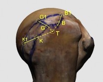
Figure 3.4. Illustration of KC measurement from the convergence point to the anterolateral points of the tendon

* Source: Research autopsy photos

 The posterolateral border of the teres minor tendon: Determined based on the landmarks of the anterolateral border of the teres minor tendon and the border of the articular cartilage.

Table 3.4. Posterior and lateral border points of the teres minor tendon

Dimensions (mm)

Average ± SD	Max	Min
KC to the anterior lateral border of the lesser rotator cuff (ZK)	23.91±3.09	31.64	19.31
KC to the edge of the articular cartilage (D 4 )	20.93 ± 2.83	26.83	15.50

3.1.2. Characteristics of the rotator cuff tendon attachment to the tuberosity

- The subscapularis tendon attachment area is not as uniform in general shape as the CX tendon attachment area to the greater tubercle of the humerus. It can be triangular in shape with one end tapering below, or comma-shaped, or oval.

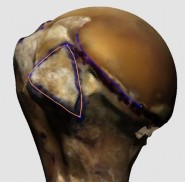
Figure 3.5. Illustration of comma-shaped, oval-shaped, and triangular subscapularis tendon attachment areas

* Source: Research autopsy photos

- The subscapularis tendon attachment area is prominent with the characteristic of widening and attaching mainly to the upper 2/3 and gradually narrowing downwards.

- If we calculate the minor tubercle in 3D space according to the above anatomical convention, then above the outer edge of the subscapularis tendon attachment area, it follows the boundary between the outer edge of the superior surface of the minor tubercle and the intertubercular groove. This area is easier to recognize. Below the tendon attachment area, it still follows the outer edge of the anterior surface of the minor tubercle and gradually moves inward.

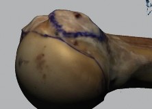
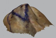
Figure 3.6. Illustration of the lateral border of the subscapularis tendon attachment superiorly and inferiorly.

* Source: Research autopsy photos

- The uppermost medial point (X) of the subscapularis attachment lies on the anterior border of the intertubercular groove and is not close to the articular cartilage border. The outermost point (Y) of the subscapularis tendon attachment also lies on the anterior border of the intertubercular groove but is located lower than the beginning of the transition zone between the upper and anterior surfaces and the anterior border of the intertubercular groove. The lowest point (Z) lies along the lateral border of the anterior surface of the lesser tubercle.

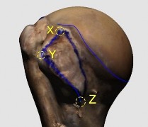
Figure 3.7. Illustration of the comma-shaped subscapular attachment area. Point X is the uppermost point, point Y is the outermost point, point Z is the lowermost point.

* Source: Research autopsy photos

- Calculate the distance between the innermost, outermost and bottommost points of the attachment area with the edge of the articular cartilage:

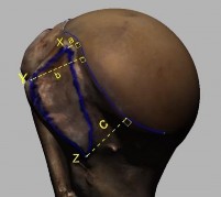
Figure 3.8. Illustration of how to measure KCs from landmarks of the subscapularis tendon attachment area

* Source: Research autopsy photos

Table 3.5. Distance between the uppermost, innermost, and lowermost points of the attachment surface to the articular cartilage margin

Dimensions (mm)

Average ± SD	Max	Min
KC (a) from the upper inner point (X) to the cartilage border joint	4.66±1.02	6.72	2.30
KC (b) from the outermost point (Y) to the shore articular cartilage	18.53±2.74	23.70	13.61
KC (c) from the bottom point (Z) to the edge of the articular cartilage	16.74±2.97	23.77	12.92

- Measure and calculate the length between the top, bottom and outermost points of the adhesion area:

Table 3.6. Length of outermost landmark to innermost and bottommost landmark of attachment area

Length (mm)

Average ± SD	Max	Min
Top outer point to top outer point inside (YX)	14.92±2.81	18.94	11.17
Top outer point to bottom point together (YZ)	24.71±2.47	29.41	21.37