b. One-line grab
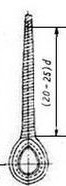
The single-wire grab bucket is suspended on a single cable 1 with a hook ring that connects with the hoisting machine's hook. The bucket is lowered into the pile of material in the open state (Case II, Figure 1.16), at which time the movable head 8 rests on the upper support head 2. Under the effect of the bucket's weight, the bucket blade 4 is deeply embedded in the pile of material. Cable 1 continues to move down and under the effect of the weight of the movable head 8, the hook 9 connects with the lower support head 6 (Case II, Figure 1.16). When cable 1 is pulled up, the bucket's jaw closes to carry out the material loading process. The bucket with the material is sealed and continues to be lifted to the position where the material needs to be unloaded.
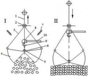
Figure 1.16: Single-line grab bucket
When it is necessary to unload the material, the lever 10 must be pushed into the stop bar 7 fixed at the height at which the material needs to be unloaded. Thus, the single-rope grab can be mounted on any type of lifting machine as long as it has a cable drum and cannot unload the material at any height.
1.4. Rope in lifting mechanism
Wires are understood as elements with a very small cross-sectional area compared to their length. Soft is understood as being easily bent in all directions, not soft and hard (measured in HB) as in Materials Science. Soft wire is understood as an element that is soft and has a certain stiffness .
a. Concept
In lifting machines, soft ropes are used to: Connect the lifting object to the lifting mechanism; Connect this object to that object and used for lashing.
b. Classification
- Synthetic cable: Endless source of raw materials, high tensile strength, less affected by the environment. Good elasticity, no need to be moisture-proof, but high cost and quickly ages over time.
- Steel cable: High tensile strength, resistant to friction, relatively low specific gravity, susceptible to corrosion...
- Plant cable: Soft, light, tough, low tensile strength, but poor abrasion resistance, high moisture absorption, swells when soaked in water, slow to dry.
- Welding chain: Large specific gravity sensitive to impacts
- Hinge chain: Often used in transmission
In lifting machines, steel cables and welded chains are often used as pulling and tying elements.
object
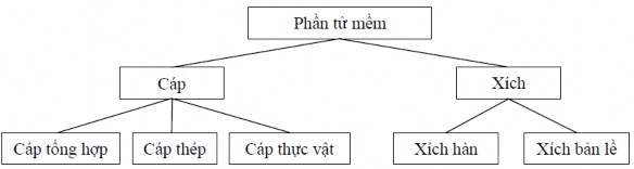
Wire classification diagram
1.4.1. Braided steel cable
a. Structure
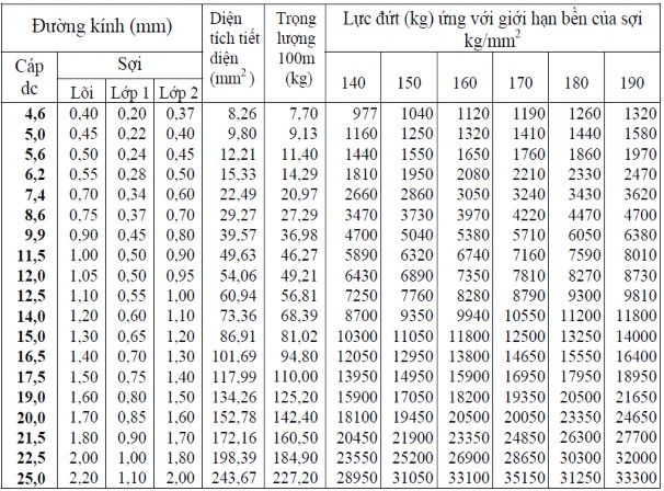
Steel cables are made from small steel wires with tensile strength up to 1800N/mm 2 and diameter from (0.2 ÷ 1) mm. To manufacture steel cables, people braid the small steel wires into "strands", and from the "strands" they braid into cables. In addition, the steel cable also has a strand made of synthetic or vegetable fibers soaked in lubricating oil to soften the cable.
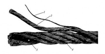
steel:
Figure 1.17: Steel cable structure
1. Steel wire; 2. Strand; 3. Cable; Steel Cable
The number of steel wires and the number of strands also affect the characteristics of the cable.
• If the cable has many steel wires:
- The cable will be soft (but the durability will not increase significantly because the outer fibers are
large shear stress).
- Poor wear resistance, easily destroyed on impact.
- High manufacturing time cost, high price.
• If the cable has multiple “strands” then:
- Flat cable surface.
- Poor compressive strength.
b. Classification
• According to manufacturing method: There are point contact cables, line cables and mixed contact cables.
fit
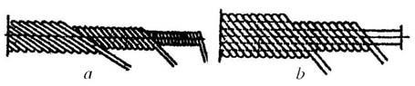
Figure 1.18: Illustration of point contact and line contact cables. a, Point contact cable; b, Line contact cable
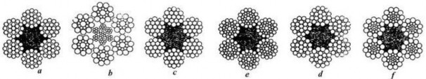
Figure 1.19: Types of line contact cables.
a. The fiber diameters are the same; b. The fiber diameters are the same in each layer.
c. Different fiber diameters in the outer layer; e. Different fiber diameters in the outer layer
d. There is a layer of steel wire as a base between the layers; f. Only the outermost layer has different fibers.
• According to the twisted form: There are regular cables and non-twisted cables.
Normal cable is a cable whose fibers and conductors are not deformed. Non-stretch cable is a cable with deformation of fibers and conductors, this cable has the following characteristics:
- Greater abrasion resistance than normal cables.
- Tension is evenly distributed.
- Has better bending resistance, hard
- Reduces wear on drums and pulleys.
• According to the twist direction: There are S cables and Z cables
- Right twisted pair cable is also known as Z cable
- Left twisted cable: Also known as S cable
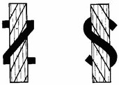
Figure 1.20: Z cable and S cable.
Note: The durability and service life of the cable are influenced by the relationship between the cable twist direction and the rotation direction of the cable drum.
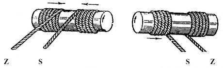
Figure 1.21: Cable twist direction and drum rotation direction
• According to braiding method: There are reverse braided cables and same-direction braided cables.
- Reverse braided cable is a type of cable in which the twist direction of the fibers in the strand and the strand in the cable are opposite.
- Same direction braided cable is the type of cable in which the twist direction of the fibers in the strand and the strand in the cable are in the same direction.
Characteristics of reverse braided cable and same-direction braided cable:
+ Reverse braided cable:
- The steel fibers are always under tension, wear increases and durability decreases.
- When not carrying a load, the spiral does not open.
+ Same direction braided cable:
- Flat surface and fuller cross-sectional area.
- Softer, more flexible and durable.
- Less wear due to increased contact surface area.
- Easy to open the twist when not carrying a load.
c. Mode, working conditions and cable calculation method
- Working conditions: Resistant to corrosion, friction and abrasion.
- Working mode: Pulling - Bending - Compressing - Twisting under the effect of tension and rotation speed.
The magnitude of the above stresses depends on many factors:
- Magnitude of applied load,
- Cable structure and diameter,
- The magnitude of friction between the fibers and the strands,
- Size and structure of the drum or pulley.
- The relationship between the twist direction of the cable and the rotation direction of the drum.
The stress state in the cable is complex. In practice, it is impossible to determine the above complicated relationship, so the cable can only be calculated approximately according to the following 3 calculation methods:
• Calculation method based on fatigue strength:
Under the simultaneous effect of the above stresses along with continuous bending and straightening during operation, the cable will become tired and eventually destroyed. Therefore, people have come to determine the limit of the number of times the cable can be bent.
The limit value of the number of times the cable can be bent depends on the value of the tension force and the ratio between the diameter of the drum (or pulley) and the diameter of the cable (D 0 = Cd c ). According to SS Torban, the ratio C will be less than 10 for plant cables and C = 15 ÷ 20 for steel cables.
DC Dutscop conducted experiments and showed that with the same load value, if C = 6.8, the cable can withstand about 10.10 3 bends before breaking, when C = 8.6, the limit of the number of bends is 45.10 3 , when C = 10.8, the limit of the number of bends is 100.10 3, when C = 12.9, the limit of the number of bends is 10.10 3 .
3
The limit of bending times is 180.10 and when C = 20.4 then after 600.10 3 bending times the cable will be destroyed.
Thus, if C is increased from 6.8 to 20.4, meaning increased 3 times, the limit of the number of bending times will increase to 60 times with the same load value.
However, the limit number of bends is difficult to calculate accurately due to the influence of many factors that are difficult to determine. Therefore, when selecting cables according to this method, it is mainly based on the dependence graphs between tension and the limit number of bends U gh experimentally.
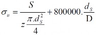
• Calculation method based on tensile and bending strength:
In practice, it is not possible to calculate all tensile, bending, compressive and torsional stresses at the same time, so the cable can only be calculated according to bending and tension, and the torsional and compressive stresses are supplemented by a reserve factor (from experiment).
When the cable is under tension S and bends around a pulley with diameter D, the steel cable has z steel wires, each with diameter d s . The following formula can be used to calculate the selection of steel cable:
• Calculation method based on breaking strength:
Nowadays, lifting machines in general, the structures and details of lifting machines in particular have been strongly standardized. Thanks to that, the calculation of steel cables will also be much simpler.
Calculation based on breaking strength is the most commonly used method of cable selection. This method is based on the maximum tension force, reserve strength coefficient and depends on the operating mode of the lifting machine to determine the cable breaking force. From the cable breaking force, we proceed to look up the cable table according to the standard (provided by the steel cable manufacturer) to select the cable.
Step 1 : Calculate S max = S dm k d (Coefficient k d is selected depending on the operating mode of the lift)
Step 2 : Calculate S d = S max n (Safety factor n = 3 ÷ 10)
Step 3 : Look up the cable selection table (See table 6).
Table 6. Soviet steel cable ΛK - 06 x 19 (Γ0CT 3077 – 55)
d. Measures to improve the durability and life of steel cables
- Use the correct load.
- Matching between rotation direction and cable twist direction, between cable diameter and drum or pulley diameter.
- Isolate the environment by covering the surface with a layer of grease.
- Coat the surface of the steel fiber with a layer of anti-corrosion material.
- Regularly grease the cable lug.
e. Connect the cable end to other machine parts
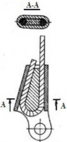
The cable end pair on the shaft needs a cable gland to protect the cable from rubbing directly on the shaft and avoid large crushing stress. The gland has a trough-shaped cross-section (Figure 1.22).
To clamp the cable end, the most commonly used method is a pair of bolts (Figure 1.22). You can also use the braiding method (Figure 1.23): unscrew the cable end, thread the fibers into the cable body, then use steel wire to wrap around the length l. This braiding method is laborious and not very sturdy, so it is rarely used.
Using a conical tube to clamp the cable ends is also very safe (figure 1.24). Thread the cable end through the small hole in the conical tube, cut the middle, bend the wires, retract, and then pour lead into the tube.
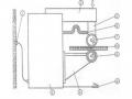
Wedge locks (Figure 1.25) are very commonly used and convenient for clamping cable ends. They can be connected and disconnected very quickly by hand without the need for specialized tools.
Figure 1.22
Figure 1.23 | |
Figure 1.24 |
Figure 1.25 |
Maybe you are interested!
-

 Illustration of Convergence Point Cx in Photographs and in 3D
 -
 Low Carbon Steel Contact Welding Mode (Single Phase AC)
 -
![Qos Assurance Methods for Multimedia Communications
zt2i3t4l5ee
zt2a3gs
zt2a3ge
zc2o3n4t5e6n7ts
low. The EF PHB requires a sufficiently large number of output ports to provide low delay, low loss, and low jitter.
EF PHBs can be implemented if the output ports bandwidth is sufficiently large, combined with small buffer sizes and other network resources dedicated to EF packets, to allow the routers service rate for EF packets on an output port to exceed the arrival rate λ of packets at that port.
This means that packets with PHB EF are considered with a pre-allocated amount of output bandwidth and a priority that ensures minimum loss, minimum delay and minimum jitter before being put into operation.
PHB EF is suitable for channel simulation, leased line simulation, and real-time services such as voice, video without compromising on high loss, delay and jitter values.
Figure 2.10 Example of EF installation
Figure 2.10 shows an example of an EF PHB implementation. This is a simple priority queue scheduling technique. At the edges of the DS domain, EF packet traffic is prioritized according to the values agreed upon by the SLA. The EF queue in the figure needs to output packets at a rate higher than the packet arrival rate λ. To provide an EF PHB over an end-to-end DS domain, bandwidth at the output ports of the core routers needs to be allocated in advance to ensure the requirement μ > λ. This can be done by a pre-configured provisioning process. In the figure, EF packets are placed in the priority queue (the upper queue). With such a length, the queue can operate with μ > λ.
Since EF was primarily used for real-time services such as voice and video, and since real-time services use UDP instead of TCP, RED is generally
not suitable for EF queues because applications using UDP will not respond to random packet drop and RED will strip unnecessary packets.
2.2.4.2 Assured Forwarding (AF) PHB
PHB AF is defined by RFC 2597. The purpose of PHB AF is to deliver packets reliably and therefore delay and jitter are considered less important than packet loss. PHB AF is suitable for non-real-time services such as applications using TCP. PHB AF first defines four classes: AF1, AF2, AF3, AF4. For each of these AF classes, packets are then classified into three subclasses with three distinct priority levels.
Table 2.8 shows the four AF classes and 12 AF subclasses and the DSCP values for the 12 AF subclasses defined by RFC 2597. RFC 2597 also allows for more than three separate priority levels to be added for internal use. However, these separate priority levels will only have internal significance.
PHB Class
PHB Subclass
Package type
DSCP
AF4
AF41
Short
100010
AF42
Medium
100100
AF43
High
100110
AF3
AF31
Short
011010
AF32
Medium
011100
AF33
High
011110
AF2
AF21
Short
010010
AF22
Medium
010100
AF23
High
010110
AF1
AF11
Short
001010
AF12
Medium
001100
AF13
High
001110
Table 2.8 AF DSCPs
The AF PHB ensures that packets are forwarded with a high probability of delivery to the destination within the bounds of the rate agreed upon in an SLA. If AF traffic at an ingress port exceeds the pre-priority rate, which is considered non-compliant or “out of profile”, the excess packets will not be delivered to the destination with the same probability as the packets belonging to the defined traffic or “in profile” packets. When there is network congestion, the out of profile packets are dropped before the in profile packets are dropped.
When service levels are defined using AF classes, different quantity and quality between AF classes can be realized by allocating different amounts of bandwidth and buffer space to the four AF classes. Unlike
EF, most AF traffic is non-real-time traffic using TCP, and the RED queue management strategy is an AQM (Adaptive Queue Management) strategy suitable for use in AF PHBs. The four AF PHB layers can be implemented as four separate queues. The output port bandwidth is divided into four AF queues. For each AF queue, packets are marked with three “colors” corresponding to three separate priority levels.
In addition to the 32 DSCP 1 groups defined in Table 2.8, 21 DSCPs have been standardized as follows: one for PHB EF, 12 for PHB AF, and 8 for CSCP. There are 11 DSCP 1 groups still available for other standards.
2.2.5.Example of Differentiated Services
We will look at an example of the Differentiated Service model and mechanism of operation. The architecture of Differentiated Service consists of two basic sets of functions:
Edge functions: include packet classification and traffic conditioning. At the inbound edge of the network, incoming packets are marked. In particular, the DS field in the packet header is set to a certain value. For example, in Figure 2.12, packets sent from H1 to H3 are marked at R1, while packets from H2 to H4 are marked at R2. The labels on the received packets identify the service class to which they belong. Different traffic classes receive different services in the core network. The RFC definition uses the term behavior aggregate rather than the term traffic class. After being marked, a packet can be forwarded immediately into the network, delayed for a period of time before being forwarded, or dropped. We will see that there are many factors that affect how a packet is marked, and whether it is forwarded immediately, delayed, or dropped.
Figure 2.12 DiffServ Example
Core functionality: When a DS-marked packet arrives at a Diffservcapable router, the packet is forwarded to the next router based on
Per-hop behavior is associated with packet classes. Per-hop behavior affects router buffers and the bandwidth shared between competing classes. An important principle of the Differentiated Service architecture is that a routers per-hop behavior is based only on the packets marking or the class to which it belongs. Therefore, if packets sent from H1 to H3 as shown in the figure receive the same marking as packets from H2 to H4, then the network routers treat the packets exactly the same, regardless of whether the packet originated from H1 or H2. For example, R3 does not distinguish between packets from h1 and H2 when forwarding packets to R4. Therefore, the Differentiated Service architecture avoids the need to maintain router state about separate source-destination pairs, which is important for network scalability.
Chapter Conclusion
Chapter 2 has presented and clarified two main models of deploying and installing quality of service in IP networks. While the traditional best-effort model has many disadvantages, later models such as IntServ and DiffServ have partly solved the problems that best-effort could not solve. IntServ follows the direction of ensuring quality of service for each separate flow, it is built similar to the circuit switching model with the use of the RSVP resource reservation protocol. IntSer is suitable for services that require fixed bandwidth that is not shared such as VoIP services, multicast TV services. However, IntSer has disadvantages such as using a lot of network resources, low scalability and lack of flexibility. DiffServ was born with the idea of solving the disadvantages of the IntServ model.
DiffServ follows the direction of ensuring quality based on the principle of hop-by-hop behavior based on the priority of marked packets. The policy for different types of traffic is decided by the administrator and can be changed according to reality, so it is very flexible. DiffServ makes better use of network resources, avoiding idle bandwidth and processing capacity on routers. In addition, the DifServ model can be deployed on many independent domains, so the ability to expand the network becomes easy.
Chapter 3: METHODS TO ENSURE QoS FOR MULTIMEDIA COMMUNICATIONS
In packet-switched networks, different packet flows often have to share the transmission medium all the way to the destination station. To ensure the fair and efficient allocation of bandwidth to flows, appropriate serving mechanisms are required at network nodes, especially at gateways or routers, where many different data flows often pass through. The scheduler is responsible for serving packets of the selected flow and deciding which packet will be served next. Here, a flow is understood as a set of packets belonging to the same priority class, or originating from the same source, or having the same source and destination addresses, etc.
In normal state when there is no congestion, packets will be sent as soon as they are delivered. In case of congestion, if QoS assurance methods are not applied, prolonged congestion can cause packet drops, affecting service quality. In some cases, congestion is prolonged and widespread in the network, which can easily lead to the network being frozen, or many packets being dropped, seriously affecting service quality.
Therefore, in this chapter, in sections 3.2 and 3.3, we introduce some typical network traffic load monitoring techniques to predict and prevent congestion before it occurs through the measure of dropping (removing) packets early when there are signs of impending congestion.
3.1. DropTail method
DropTail is a simple, traditional queue management method based on FIFO mechanism. All incoming packets are placed in the queue, when the queue is full, the later packets are dropped.
Due to its simplicity and ease of implementation, DropTail has been used for many years on Internet router systems. However, this algorithm has the following disadvantages:
− Cannot avoid the phenomenon of “Lock out”: Occurs when 1 or several traffic streams monopolize the queue, making packets of other connections unable to pass through the router. This phenomenon greatly affects reliable transmission protocols such as TCP. According to the anti-congestion algorithm, when locked out, the TCP connection stream will reduce the window size and reduce the packet transmission speed exponentially.
− Can cause Global Synchronization: This is the result of a severe “Lock out” phenomenon. Some neighboring routers have their queues monopolized by a number of connections, causing a series of other TCP connections to be unable to pass through and simultaneously reducing the transmission speed. After those monopolized connections are temporarily suspended,
Once the queue is cleared, it takes a considerable amount of time for TCP connections to return to their original speed.
− Full Queue phenomenon: Data transmitted on the Internet often has an explosion, packets arriving at the router are often in clusters rather than in turn. Therefore, the operating mechanism of DropTail makes the queue easily full for a long period of time, leading to the average delay time of large packets. To avoid this phenomenon, with DropTail, the only way is to increase the routers buffer, this method is very expensive and ineffective.
− No QoS guarantee: With the DropTail mechanism, there is no way to prioritize important packets to be transmitted through the router earlier when all are in the queue. Meanwhile, with multimedia communication, ensuring connection and stable speed is extremely important and the DropTail algorithm cannot satisfy.
The problem of choosing the buffer size of the routers in the network is to “absorb” short bursts of traffic without causing too much queuing delay. This is necessary in bursty data transmission. The queue size determines the size of the packet bursts (traffic spikes) that we want to be able to transmit without being dropped at the routers.
In IP-based application networks, packet dropping is an important mechanism for indirectly reporting congestion to end stations. A solution that prevents router queues from filling up while reducing the packet drop rate is called dynamic queue management.
3.2. Random elimination method – RED
3.2.1 Overview
RED (Random Early Detection of congestion; Random Early Drop) is one of the first AQM algorithms proposed in 1993 by Sally Floyd and Van Jacobson, two scientists at the Lawrence Berkeley Laboratory of the University of California, USA. Due to its outstanding advantages compared to previous queue management algorithms, RED has been widely installed and deployed on the Internet.
The most fundamental point of their work is that the most effective place to detect congestion and react to it is at the gateway or router.
Source entities (senders) can also do this by estimating end-to-end delay, throughput variability, or the rate of packet retransmissions due to drop. However, the sender and receiver view of a particular connection cannot tell which gateways on the network are congested, and cannot distinguish between propagation delay and queuing delay. Only the gateway has a true view of the state of the queue, the link share of the connections passing through it at any given time, and the quality of service requirements of the
traffic flows. The RED gateway monitors the average queue length, which detects early signs of impending congestion (average queue length exceeding a predetermined threshold) and reacts appropriately in one of two ways:
− Drop incoming packets with a certain probability, to indirectly inform the source of congestion, the source needs to reduce the transmission rate to keep the queue from filling up, maintaining the ability to absorb incoming traffic spikes.
− Mark “congestion” with a certain probability in the ECN field in the header of TCP packets to notify the source (the receiving entity will copy this bit into the acknowledgement packet).
Figure 3. 1 RED algorithm
The main goal of RED is to avoid congestion by keeping the average queue size within a sufficiently small and stable region, which also means keeping the queuing delay sufficiently small and stable. Achieving this goal also helps: avoid global synchronization, not resist bursty traffic flows (i.e. flows with low average throughput but high volatility), and maintain an upper bound on the average queue size even in the absence of cooperation from transport layer protocols.
To achieve the above goals, RED gateways must do the following:
− The first is to detect congestion early and react appropriately to keep the average queue size small enough to keep the network operating in the low latency, high throughput region, while still allowing the queue size to fluctuate within a certain range to absorb short-term fluctuations. As discussed above, the gateway is the most appropriate place to detect congestion and is also the most appropriate place to decide which specific connection to report congestion to.
− The second thing is to notify the source of congestion. This is done by marking and notifying the source to reduce traffic. Normally the RED gateway will randomly drop packets. However, if congestion
If congestion is detected before the queue is full, it should be combined with packet marking to signal congestion. The RED gateway has two options: drop or mark; where marking is done by marking the ECN field of the packet with a certain probability, to signal the source to reduce the traffic entering the network.
− An important goal that RED gateways need to achieve is to avoid global synchronization and not to resist traffic flows that have a sudden characteristic. Global synchronization occurs when all connections simultaneously reduce their transmission window size, leading to a severe drop in throughput at the same time. On the other hand, Drop Tail or Random Drop strategies are very sensitive to sudden flows; that is, the gateway queue will often overflow when packets from these flows arrive. To avoid these two phenomena, gateways can use special algorithms to detect congestion and decide which connections will be notified of congestion at the gateway. The RED gateway randomly selects incoming packets to mark; with this method, the probability of marking a packet from a particular connection is proportional to the connections shared bandwidth at the gateway.
− Another goal is to control the average queue size even without cooperation from the source entities. This can be done by dropping packets when the average size exceeds an upper threshold (instead of marking it). This approach is necessary in cases where most connections have transmission times that are less than the round-trip time, or where the source entities are not able to reduce traffic in response to marking or dropping packets (such as UDP flows).
3.2.2 Algorithm
This section describes the algorithm for RED gateways. RED gateways calculate the average queue size using a low-pass filter. This average queue size is compared with two thresholds: minth and maxth. When the average queue size is less than the lower threshold, no incoming packets are marked or dropped; when the average queue size is greater than the upper threshold, all incoming packets are dropped. When the average queue size is between minth and maxth, each incoming packet is marked or dropped with a probability pa, where pa is a function of the average queue size avg; the probability of marking or dropping a packet for a particular connection is proportional to the bandwidth share of that connection at the gateway. The general algorithm for a RED gateway is described as follows: [5]
For each packet arrival
Caculate the average queue size avg If minth ≤ avg < maxth
div.maincontent .s1 { color: black; font-family:Times New Roman, serif; font-style: normal; font-weight: normal; text-decoration: none; font-size: 15pt; }
div.maincontent .s2 { color: black; font-family:Times New Roman, serif; font-style: normal; font-weight: bold; text-decoration: none; font-size: 15pt; }
div.maincontent .p { color: black; font-family:Times New Roman, serif; font-style: normal; font-weight: normal; text-decoration: none; font-size: 14pt; margin:0pt; }
div.maincontent p { color: black; font-family:Times New Roman, serif; font-style: normal; font-weight: normal; text-decoration: none; font-size: 14pt; margin:0pt; }
div.maincontent .s3 { color: black; font-family:Times New Roman, serif; font-style: normal; font-weight: bold; text-decoration: none; font-size: 14pt; }
div.maincontent .s4 { color: black; font-family:Times New Roman, serif; font-style: normal; font-weight: normal; text-decoration: none; font-size: 14pt; }
div.maincontent .s5 { color: black; font-family:Times New Roman, serif; font-style: italic; font-weight: normal; text-decoration: none; font-size: 14pt; }
div.maincontent .s6 { color: black; font-family:Times New Roman, serif; font-style: italic; font-weight: bold; text-decoration: none; font-size: 14pt; }
div.maincontent .s7 { color: black; font-family:Wingdings; font-style: normal; font-weight: normal; text-decoration: none; font-size: 14pt; }
div.maincontent .s8 { color: black; font-family:Arial, sans-serif; font-style: italic; font-weight: bold; text-decoration: none; font-size: 15pt; }
div.maincontent .s9 { color: black; font-family:Times New Roman, serif; font-style: normal; font-weight: bold; text-decoration: none; font-size: 14pt; }
div.maincontent .s10 { color: black; font-family:Times New Roman, serif; font-style: normal; font-weight: normal; text-decoration: none; font-size: 9pt; vertical-align: 6pt; }
div.maincontent .s11 { color: black; font-family:Times New Roman, serif; font-style: normal; font-weight: normal; text-decoration: none; font-size: 13pt; }
div.maincontent .s12 { color: black; font-family:Times New Roman, serif; font-style: normal; font-weight: normal; text-decoration: none; font-size: 10pt; }
div.maincontent .s13 { color: black; font-family:Times New Roman, serif; font-style: normal; font-weight: normal; text-d](https://tailieuthamkhao.com/uploads/2022/05/15/danh-gia-hieu-qua-dam-bao-qos-cho-truyen-thong-da-phuong-tien-cua-chien-6-1-120x90.jpg) Qos Assurance Methods for Multimedia Communications
zt2i3t4l5ee
zt2a3gs
zt2a3ge
zc2o3n4t5e6n7ts
low. The EF PHB requires a sufficiently large number of output ports to provide low delay, low loss, and low jitter.
EF PHBs can be implemented if the output port's bandwidth is sufficiently large, combined with small buffer sizes and other network resources dedicated to EF packets, to allow the router's service rate for EF packets on an output port to exceed the arrival rate λ of packets at that port.
This means that packets with PHB EF are considered with a pre-allocated amount of output bandwidth and a priority that ensures minimum loss, minimum delay and minimum jitter before being put into operation.
PHB EF is suitable for channel simulation, leased line simulation, and real-time services such as voice, video without compromising on high loss, delay and jitter values.
Figure 2.10 Example of EF installation
Figure 2.10 shows an example of an EF PHB implementation. This is a simple priority queue scheduling technique. At the edges of the DS domain, EF packet traffic is prioritized according to the values agreed upon by the SLA. The EF queue in the figure needs to output packets at a rate higher than the packet arrival rate λ. To provide an EF PHB over an end-to-end DS domain, bandwidth at the output ports of the core routers needs to be allocated in advance to ensure the requirement μ > λ. This can be done by a pre-configured provisioning process. In the figure, EF packets are placed in the priority queue (the upper queue). With such a length, the queue can operate with μ > λ.
Since EF was primarily used for real-time services such as voice and video, and since real-time services use UDP instead of TCP, RED is generally
not suitable for EF queues because applications using UDP will not respond to random packet drop and RED will strip unnecessary packets.
2.2.4.2 Assured Forwarding (AF) PHB
PHB AF is defined by RFC 2597. The purpose of PHB AF is to deliver packets reliably and therefore delay and jitter are considered less important than packet loss. PHB AF is suitable for non-real-time services such as applications using TCP. PHB AF first defines four classes: AF1, AF2, AF3, AF4. For each of these AF classes, packets are then classified into three subclasses with three distinct priority levels.
Table 2.8 shows the four AF classes and 12 AF subclasses and the DSCP values for the 12 AF subclasses defined by RFC 2597. RFC 2597 also allows for more than three separate priority levels to be added for internal use. However, these separate priority levels will only have internal significance.
PHB Class
PHB Subclass
Package type
DSCP
AF4
AF41
Short
100010
AF42
Medium
100100
AF43
High
100110
AF3
AF31
Short
011010
AF32
Medium
011100
AF33
High
011110
AF2
AF21
Short
010010
AF22
Medium
010100
AF23
High
010110
AF1
AF11
Short
001010
AF12
Medium
001100
AF13
High
001110
Table 2.8 AF DSCPs
The AF PHB ensures that packets are forwarded with a high probability of delivery to the destination within the bounds of the rate agreed upon in an SLA. If AF traffic at an ingress port exceeds the pre-priority rate, which is considered non-compliant or “out of profile”, the excess packets will not be delivered to the destination with the same probability as the packets belonging to the defined traffic or “in profile” packets. When there is network congestion, the out of profile packets are dropped before the in profile packets are dropped.
When service levels are defined using AF classes, different quantity and quality between AF classes can be realized by allocating different amounts of bandwidth and buffer space to the four AF classes. Unlike
EF, most AF traffic is non-real-time traffic using TCP, and the RED queue management strategy is an AQM (Adaptive Queue Management) strategy suitable for use in AF PHBs. The four AF PHB layers can be implemented as four separate queues. The output port bandwidth is divided into four AF queues. For each AF queue, packets are marked with three “colors” corresponding to three separate priority levels.
In addition to the 32 DSCP 1 groups defined in Table 2.8, 21 DSCPs have been standardized as follows: one for PHB EF, 12 for PHB AF, and 8 for CSCP. There are 11 DSCP 1 groups still available for other standards.
2.2.5.Example of Differentiated Services
We will look at an example of the Differentiated Service model and mechanism of operation. The architecture of Differentiated Service consists of two basic sets of functions:
Edge functions: include packet classification and traffic conditioning. At the inbound edge of the network, incoming packets are marked. In particular, the DS field in the packet header is set to a certain value. For example, in Figure 2.12, packets sent from H1 to H3 are marked at R1, while packets from H2 to H4 are marked at R2. The labels on the received packets identify the service class to which they belong. Different traffic classes receive different services in the core network. The RFC definition uses the term behavior aggregate rather than the term traffic class. After being marked, a packet can be forwarded immediately into the network, delayed for a period of time before being forwarded, or dropped. We will see that there are many factors that affect how a packet is marked, and whether it is forwarded immediately, delayed, or dropped.
Figure 2.12 DiffServ Example
Core functionality: When a DS-marked packet arrives at a Diffservcapable router, the packet is forwarded to the next router based on
Per-hop behavior is associated with packet classes. Per-hop behavior affects router buffers and the bandwidth shared between competing classes. An important principle of the Differentiated Service architecture is that a router's per-hop behavior is based only on the packet's marking or the class to which it belongs. Therefore, if packets sent from H1 to H3 as shown in the figure receive the same marking as packets from H2 to H4, then the network routers treat the packets exactly the same, regardless of whether the packet originated from H1 or H2. For example, R3 does not distinguish between packets from h1 and H2 when forwarding packets to R4. Therefore, the Differentiated Service architecture avoids the need to maintain router state about separate source-destination pairs, which is important for network scalability.
Chapter Conclusion
Chapter 2 has presented and clarified two main models of deploying and installing quality of service in IP networks. While the traditional best-effort model has many disadvantages, later models such as IntServ and DiffServ have partly solved the problems that best-effort could not solve. IntServ follows the direction of ensuring quality of service for each separate flow, it is built similar to the circuit switching model with the use of the RSVP resource reservation protocol. IntSer is suitable for services that require fixed bandwidth that is not shared such as VoIP services, multicast TV services. However, IntSer has disadvantages such as using a lot of network resources, low scalability and lack of flexibility. DiffServ was born with the idea of solving the disadvantages of the IntServ model.
DiffServ follows the direction of ensuring quality based on the principle of hop-by-hop behavior based on the priority of marked packets. The policy for different types of traffic is decided by the administrator and can be changed according to reality, so it is very flexible. DiffServ makes better use of network resources, avoiding idle bandwidth and processing capacity on routers. In addition, the DifServ model can be deployed on many independent domains, so the ability to expand the network becomes easy.
Chapter 3: METHODS TO ENSURE QoS FOR MULTIMEDIA COMMUNICATIONS
In packet-switched networks, different packet flows often have to share the transmission medium all the way to the destination station. To ensure the fair and efficient allocation of bandwidth to flows, appropriate serving mechanisms are required at network nodes, especially at gateways or routers, where many different data flows often pass through. The scheduler is responsible for serving packets of the selected flow and deciding which packet will be served next. Here, a flow is understood as a set of packets belonging to the same priority class, or originating from the same source, or having the same source and destination addresses, etc.
In normal state when there is no congestion, packets will be sent as soon as they are delivered. In case of congestion, if QoS assurance methods are not applied, prolonged congestion can cause packet drops, affecting service quality. In some cases, congestion is prolonged and widespread in the network, which can easily lead to the network being "frozen", or many packets being dropped, seriously affecting service quality.
Therefore, in this chapter, in sections 3.2 and 3.3, we introduce some typical network traffic load monitoring techniques to predict and prevent congestion before it occurs through the measure of dropping (removing) packets early when there are signs of impending congestion.
3.1. DropTail method
DropTail is a simple, traditional queue management method based on FIFO mechanism. All incoming packets are placed in the queue, when the queue is full, the later packets are dropped.
Due to its simplicity and ease of implementation, DropTail has been used for many years on Internet router systems. However, this algorithm has the following disadvantages:
− Cannot avoid the phenomenon of “Lock out”: Occurs when 1 or several traffic streams monopolize the queue, making packets of other connections unable to pass through the router. This phenomenon greatly affects reliable transmission protocols such as TCP. According to the anti-congestion algorithm, when locked out, the TCP connection stream will reduce the window size and reduce the packet transmission speed exponentially.
− Can cause Global Synchronization: This is the result of a severe “Lock out” phenomenon. Some neighboring routers have their queues monopolized by a number of connections, causing a series of other TCP connections to be unable to pass through and simultaneously reducing the transmission speed. After those monopolized connections are temporarily suspended,
Once the queue is cleared, it takes a considerable amount of time for TCP connections to return to their original speed.
− Full Queue phenomenon: Data transmitted on the Internet often has an explosion, packets arriving at the router are often in clusters rather than in turn. Therefore, the operating mechanism of DropTail makes the queue easily full for a long period of time, leading to the average delay time of large packets. To avoid this phenomenon, with DropTail, the only way is to increase the router's buffer, this method is very expensive and ineffective.
− No QoS guarantee: With the DropTail mechanism, there is no way to prioritize important packets to be transmitted through the router earlier when all are in the queue. Meanwhile, with multimedia communication, ensuring connection and stable speed is extremely important and the DropTail algorithm cannot satisfy.
The problem of choosing the buffer size of the routers in the network is to “absorb” short bursts of traffic without causing too much queuing delay. This is necessary in bursty data transmission. The queue size determines the size of the packet bursts (traffic spikes) that we want to be able to transmit without being dropped at the routers.
In IP-based application networks, packet dropping is an important mechanism for indirectly reporting congestion to end stations. A solution that prevents router queues from filling up while reducing the packet drop rate is called dynamic queue management.
3.2. Random elimination method – RED
3.2.1 Overview
RED (Random Early Detection of congestion; Random Early Drop) is one of the first AQM algorithms proposed in 1993 by Sally Floyd and Van Jacobson, two scientists at the Lawrence Berkeley Laboratory of the University of California, USA. Due to its outstanding advantages compared to previous queue management algorithms, RED has been widely installed and deployed on the Internet.
The most fundamental point of their work is that the most effective place to detect congestion and react to it is at the gateway or router.
Source entities (senders) can also do this by estimating end-to-end delay, throughput variability, or the rate of packet retransmissions due to drop. However, the sender and receiver view of a particular connection cannot tell which gateways on the network are congested, and cannot distinguish between propagation delay and queuing delay. Only the gateway has a true view of the state of the queue, the link share of the connections passing through it at any given time, and the quality of service requirements of the
traffic flows. The RED gateway monitors the average queue length, which detects early signs of impending congestion (average queue length exceeding a predetermined threshold) and reacts appropriately in one of two ways:
− Drop incoming packets with a certain probability, to indirectly inform the source of congestion, the source needs to reduce the transmission rate to keep the queue from filling up, maintaining the ability to absorb incoming traffic spikes.
− Mark “congestion” with a certain probability in the ECN field in the header of TCP packets to notify the source (the receiving entity will copy this bit into the acknowledgement packet).
Figure 3. 1 RED algorithm
The main goal of RED is to avoid congestion by keeping the average queue size within a sufficiently small and stable region, which also means keeping the queuing delay sufficiently small and stable. Achieving this goal also helps: avoid global synchronization, not resist bursty traffic flows (i.e. flows with low average throughput but high volatility), and maintain an upper bound on the average queue size even in the absence of cooperation from transport layer protocols.
To achieve the above goals, RED gateways must do the following:
− The first is to detect congestion early and react appropriately to keep the average queue size small enough to keep the network operating in the low latency, high throughput region, while still allowing the queue size to fluctuate within a certain range to absorb short-term fluctuations. As discussed above, the gateway is the most appropriate place to detect congestion and is also the most appropriate place to decide which specific connection to report congestion to.
− The second thing is to notify the source of congestion. This is done by marking and notifying the source to reduce traffic. Normally the RED gateway will randomly drop packets. However, if congestion
If congestion is detected before the queue is full, it should be combined with packet marking to signal congestion. The RED gateway has two options: drop or mark; where marking is done by marking the ECN field of the packet with a certain probability, to signal the source to reduce the traffic entering the network.
− An important goal that RED gateways need to achieve is to avoid global synchronization and not to resist traffic flows that have a sudden characteristic. Global synchronization occurs when all connections simultaneously reduce their transmission window size, leading to a severe drop in throughput at the same time. On the other hand, Drop Tail or Random Drop strategies are very sensitive to sudden flows; that is, the gateway queue will often overflow when packets from these flows arrive. To avoid these two phenomena, gateways can use special algorithms to detect congestion and decide which connections will be notified of congestion at the gateway. The RED gateway randomly selects incoming packets to mark; with this method, the probability of marking a packet from a particular connection is proportional to the connection's shared bandwidth at the gateway.
− Another goal is to control the average queue size even without cooperation from the source entities. This can be done by dropping packets when the average size exceeds an upper threshold (instead of marking it). This approach is necessary in cases where most connections have transmission times that are less than the round-trip time, or where the source entities are not able to reduce traffic in response to marking or dropping packets (such as UDP flows).
3.2.2 Algorithm
This section describes the algorithm for RED gateways. RED gateways calculate the average queue size using a low-pass filter. This average queue size is compared with two thresholds: minth and maxth. When the average queue size is less than the lower threshold, no incoming packets are marked or dropped; when the average queue size is greater than the upper threshold, all incoming packets are dropped. When the average queue size is between minth and maxth, each incoming packet is marked or dropped with a probability pa, where pa is a function of the average queue size avg; the probability of marking or dropping a packet for a particular connection is proportional to the bandwidth share of that connection at the gateway. The general algorithm for a RED gateway is described as follows: [5]
For each packet arrival
Caculate the average queue size avg If minth ≤ avg < maxth
div.maincontent .s1 { color: black; font-family:"Times New Roman", serif; font-style: normal; font-weight: normal; text-decoration: none; font-size: 15pt; }
div.maincontent .s2 { color: black; font-family:"Times New Roman", serif; font-style: normal; font-weight: bold; text-decoration: none; font-size: 15pt; }
div.maincontent .p { color: black; font-family:"Times New Roman", serif; font-style: normal; font-weight: normal; text-decoration: none; font-size: 14pt; margin:0pt; }
div.maincontent p { color: black; font-family:"Times New Roman", serif; font-style: normal; font-weight: normal; text-decoration: none; font-size: 14pt; margin:0pt; }
div.maincontent .s3 { color: black; font-family:"Times New Roman", serif; font-style: normal; font-weight: bold; text-decoration: none; font-size: 14pt; }
div.maincontent .s4 { color: black; font-family:"Times New Roman", serif; font-style: normal; font-weight: normal; text-decoration: none; font-size: 14pt; }
div.maincontent .s5 { color: black; font-family:"Times New Roman", serif; font-style: italic; font-weight: normal; text-decoration: none; font-size: 14pt; }
div.maincontent .s6 { color: black; font-family:"Times New Roman", serif; font-style: italic; font-weight: bold; text-decoration: none; font-size: 14pt; }
div.maincontent .s7 { color: black; font-family:Wingdings; font-style: normal; font-weight: normal; text-decoration: none; font-size: 14pt; }
div.maincontent .s8 { color: black; font-family:Arial, sans-serif; font-style: italic; font-weight: bold; text-decoration: none; font-size: 15pt; }
div.maincontent .s9 { color: black; font-family:"Times New Roman", serif; font-style: normal; font-weight: bold; text-decoration: none; font-size: 14pt; }
div.maincontent .s10 { color: black; font-family:"Times New Roman", serif; font-style: normal; font-weight: normal; text-decoration: none; font-size: 9pt; vertical-align: 6pt; }
div.maincontent .s11 { color: black; font-family:"Times New Roman", serif; font-style: normal; font-weight: normal; text-decoration: none; font-size: 13pt; }
div.maincontent .s12 { color: black; font-family:"Times New Roman", serif; font-style: normal; font-weight: normal; text-decoration: none; font-size: 10pt; }
div.maincontent .s13 { color: black; font-family:"Times New Roman", serif; font-style: normal; font-weight: normal; text-d
Qos Assurance Methods for Multimedia Communications
zt2i3t4l5ee
zt2a3gs
zt2a3ge
zc2o3n4t5e6n7ts
low. The EF PHB requires a sufficiently large number of output ports to provide low delay, low loss, and low jitter.
EF PHBs can be implemented if the output port's bandwidth is sufficiently large, combined with small buffer sizes and other network resources dedicated to EF packets, to allow the router's service rate for EF packets on an output port to exceed the arrival rate λ of packets at that port.
This means that packets with PHB EF are considered with a pre-allocated amount of output bandwidth and a priority that ensures minimum loss, minimum delay and minimum jitter before being put into operation.
PHB EF is suitable for channel simulation, leased line simulation, and real-time services such as voice, video without compromising on high loss, delay and jitter values.
Figure 2.10 Example of EF installation
Figure 2.10 shows an example of an EF PHB implementation. This is a simple priority queue scheduling technique. At the edges of the DS domain, EF packet traffic is prioritized according to the values agreed upon by the SLA. The EF queue in the figure needs to output packets at a rate higher than the packet arrival rate λ. To provide an EF PHB over an end-to-end DS domain, bandwidth at the output ports of the core routers needs to be allocated in advance to ensure the requirement μ > λ. This can be done by a pre-configured provisioning process. In the figure, EF packets are placed in the priority queue (the upper queue). With such a length, the queue can operate with μ > λ.
Since EF was primarily used for real-time services such as voice and video, and since real-time services use UDP instead of TCP, RED is generally
not suitable for EF queues because applications using UDP will not respond to random packet drop and RED will strip unnecessary packets.
2.2.4.2 Assured Forwarding (AF) PHB
PHB AF is defined by RFC 2597. The purpose of PHB AF is to deliver packets reliably and therefore delay and jitter are considered less important than packet loss. PHB AF is suitable for non-real-time services such as applications using TCP. PHB AF first defines four classes: AF1, AF2, AF3, AF4. For each of these AF classes, packets are then classified into three subclasses with three distinct priority levels.
Table 2.8 shows the four AF classes and 12 AF subclasses and the DSCP values for the 12 AF subclasses defined by RFC 2597. RFC 2597 also allows for more than three separate priority levels to be added for internal use. However, these separate priority levels will only have internal significance.
PHB Class
PHB Subclass
Package type
DSCP
AF4
AF41
Short
100010
AF42
Medium
100100
AF43
High
100110
AF3
AF31
Short
011010
AF32
Medium
011100
AF33
High
011110
AF2
AF21
Short
010010
AF22
Medium
010100
AF23
High
010110
AF1
AF11
Short
001010
AF12
Medium
001100
AF13
High
001110
Table 2.8 AF DSCPs
The AF PHB ensures that packets are forwarded with a high probability of delivery to the destination within the bounds of the rate agreed upon in an SLA. If AF traffic at an ingress port exceeds the pre-priority rate, which is considered non-compliant or “out of profile”, the excess packets will not be delivered to the destination with the same probability as the packets belonging to the defined traffic or “in profile” packets. When there is network congestion, the out of profile packets are dropped before the in profile packets are dropped.
When service levels are defined using AF classes, different quantity and quality between AF classes can be realized by allocating different amounts of bandwidth and buffer space to the four AF classes. Unlike
EF, most AF traffic is non-real-time traffic using TCP, and the RED queue management strategy is an AQM (Adaptive Queue Management) strategy suitable for use in AF PHBs. The four AF PHB layers can be implemented as four separate queues. The output port bandwidth is divided into four AF queues. For each AF queue, packets are marked with three “colors” corresponding to three separate priority levels.
In addition to the 32 DSCP 1 groups defined in Table 2.8, 21 DSCPs have been standardized as follows: one for PHB EF, 12 for PHB AF, and 8 for CSCP. There are 11 DSCP 1 groups still available for other standards.
2.2.5.Example of Differentiated Services
We will look at an example of the Differentiated Service model and mechanism of operation. The architecture of Differentiated Service consists of two basic sets of functions:
Edge functions: include packet classification and traffic conditioning. At the inbound edge of the network, incoming packets are marked. In particular, the DS field in the packet header is set to a certain value. For example, in Figure 2.12, packets sent from H1 to H3 are marked at R1, while packets from H2 to H4 are marked at R2. The labels on the received packets identify the service class to which they belong. Different traffic classes receive different services in the core network. The RFC definition uses the term behavior aggregate rather than the term traffic class. After being marked, a packet can be forwarded immediately into the network, delayed for a period of time before being forwarded, or dropped. We will see that there are many factors that affect how a packet is marked, and whether it is forwarded immediately, delayed, or dropped.
Figure 2.12 DiffServ Example
Core functionality: When a DS-marked packet arrives at a Diffservcapable router, the packet is forwarded to the next router based on
Per-hop behavior is associated with packet classes. Per-hop behavior affects router buffers and the bandwidth shared between competing classes. An important principle of the Differentiated Service architecture is that a router's per-hop behavior is based only on the packet's marking or the class to which it belongs. Therefore, if packets sent from H1 to H3 as shown in the figure receive the same marking as packets from H2 to H4, then the network routers treat the packets exactly the same, regardless of whether the packet originated from H1 or H2. For example, R3 does not distinguish between packets from h1 and H2 when forwarding packets to R4. Therefore, the Differentiated Service architecture avoids the need to maintain router state about separate source-destination pairs, which is important for network scalability.
Chapter Conclusion
Chapter 2 has presented and clarified two main models of deploying and installing quality of service in IP networks. While the traditional best-effort model has many disadvantages, later models such as IntServ and DiffServ have partly solved the problems that best-effort could not solve. IntServ follows the direction of ensuring quality of service for each separate flow, it is built similar to the circuit switching model with the use of the RSVP resource reservation protocol. IntSer is suitable for services that require fixed bandwidth that is not shared such as VoIP services, multicast TV services. However, IntSer has disadvantages such as using a lot of network resources, low scalability and lack of flexibility. DiffServ was born with the idea of solving the disadvantages of the IntServ model.
DiffServ follows the direction of ensuring quality based on the principle of hop-by-hop behavior based on the priority of marked packets. The policy for different types of traffic is decided by the administrator and can be changed according to reality, so it is very flexible. DiffServ makes better use of network resources, avoiding idle bandwidth and processing capacity on routers. In addition, the DifServ model can be deployed on many independent domains, so the ability to expand the network becomes easy.
Chapter 3: METHODS TO ENSURE QoS FOR MULTIMEDIA COMMUNICATIONS
In packet-switched networks, different packet flows often have to share the transmission medium all the way to the destination station. To ensure the fair and efficient allocation of bandwidth to flows, appropriate serving mechanisms are required at network nodes, especially at gateways or routers, where many different data flows often pass through. The scheduler is responsible for serving packets of the selected flow and deciding which packet will be served next. Here, a flow is understood as a set of packets belonging to the same priority class, or originating from the same source, or having the same source and destination addresses, etc.
In normal state when there is no congestion, packets will be sent as soon as they are delivered. In case of congestion, if QoS assurance methods are not applied, prolonged congestion can cause packet drops, affecting service quality. In some cases, congestion is prolonged and widespread in the network, which can easily lead to the network being "frozen", or many packets being dropped, seriously affecting service quality.
Therefore, in this chapter, in sections 3.2 and 3.3, we introduce some typical network traffic load monitoring techniques to predict and prevent congestion before it occurs through the measure of dropping (removing) packets early when there are signs of impending congestion.
3.1. DropTail method
DropTail is a simple, traditional queue management method based on FIFO mechanism. All incoming packets are placed in the queue, when the queue is full, the later packets are dropped.
Due to its simplicity and ease of implementation, DropTail has been used for many years on Internet router systems. However, this algorithm has the following disadvantages:
− Cannot avoid the phenomenon of “Lock out”: Occurs when 1 or several traffic streams monopolize the queue, making packets of other connections unable to pass through the router. This phenomenon greatly affects reliable transmission protocols such as TCP. According to the anti-congestion algorithm, when locked out, the TCP connection stream will reduce the window size and reduce the packet transmission speed exponentially.
− Can cause Global Synchronization: This is the result of a severe “Lock out” phenomenon. Some neighboring routers have their queues monopolized by a number of connections, causing a series of other TCP connections to be unable to pass through and simultaneously reducing the transmission speed. After those monopolized connections are temporarily suspended,
Once the queue is cleared, it takes a considerable amount of time for TCP connections to return to their original speed.
− Full Queue phenomenon: Data transmitted on the Internet often has an explosion, packets arriving at the router are often in clusters rather than in turn. Therefore, the operating mechanism of DropTail makes the queue easily full for a long period of time, leading to the average delay time of large packets. To avoid this phenomenon, with DropTail, the only way is to increase the router's buffer, this method is very expensive and ineffective.
− No QoS guarantee: With the DropTail mechanism, there is no way to prioritize important packets to be transmitted through the router earlier when all are in the queue. Meanwhile, with multimedia communication, ensuring connection and stable speed is extremely important and the DropTail algorithm cannot satisfy.
The problem of choosing the buffer size of the routers in the network is to “absorb” short bursts of traffic without causing too much queuing delay. This is necessary in bursty data transmission. The queue size determines the size of the packet bursts (traffic spikes) that we want to be able to transmit without being dropped at the routers.
In IP-based application networks, packet dropping is an important mechanism for indirectly reporting congestion to end stations. A solution that prevents router queues from filling up while reducing the packet drop rate is called dynamic queue management.
3.2. Random elimination method – RED
3.2.1 Overview
RED (Random Early Detection of congestion; Random Early Drop) is one of the first AQM algorithms proposed in 1993 by Sally Floyd and Van Jacobson, two scientists at the Lawrence Berkeley Laboratory of the University of California, USA. Due to its outstanding advantages compared to previous queue management algorithms, RED has been widely installed and deployed on the Internet.
The most fundamental point of their work is that the most effective place to detect congestion and react to it is at the gateway or router.
Source entities (senders) can also do this by estimating end-to-end delay, throughput variability, or the rate of packet retransmissions due to drop. However, the sender and receiver view of a particular connection cannot tell which gateways on the network are congested, and cannot distinguish between propagation delay and queuing delay. Only the gateway has a true view of the state of the queue, the link share of the connections passing through it at any given time, and the quality of service requirements of the
traffic flows. The RED gateway monitors the average queue length, which detects early signs of impending congestion (average queue length exceeding a predetermined threshold) and reacts appropriately in one of two ways:
− Drop incoming packets with a certain probability, to indirectly inform the source of congestion, the source needs to reduce the transmission rate to keep the queue from filling up, maintaining the ability to absorb incoming traffic spikes.
− Mark “congestion” with a certain probability in the ECN field in the header of TCP packets to notify the source (the receiving entity will copy this bit into the acknowledgement packet).
Figure 3. 1 RED algorithm
The main goal of RED is to avoid congestion by keeping the average queue size within a sufficiently small and stable region, which also means keeping the queuing delay sufficiently small and stable. Achieving this goal also helps: avoid global synchronization, not resist bursty traffic flows (i.e. flows with low average throughput but high volatility), and maintain an upper bound on the average queue size even in the absence of cooperation from transport layer protocols.
To achieve the above goals, RED gateways must do the following:
− The first is to detect congestion early and react appropriately to keep the average queue size small enough to keep the network operating in the low latency, high throughput region, while still allowing the queue size to fluctuate within a certain range to absorb short-term fluctuations. As discussed above, the gateway is the most appropriate place to detect congestion and is also the most appropriate place to decide which specific connection to report congestion to.
− The second thing is to notify the source of congestion. This is done by marking and notifying the source to reduce traffic. Normally the RED gateway will randomly drop packets. However, if congestion
If congestion is detected before the queue is full, it should be combined with packet marking to signal congestion. The RED gateway has two options: drop or mark; where marking is done by marking the ECN field of the packet with a certain probability, to signal the source to reduce the traffic entering the network.
− An important goal that RED gateways need to achieve is to avoid global synchronization and not to resist traffic flows that have a sudden characteristic. Global synchronization occurs when all connections simultaneously reduce their transmission window size, leading to a severe drop in throughput at the same time. On the other hand, Drop Tail or Random Drop strategies are very sensitive to sudden flows; that is, the gateway queue will often overflow when packets from these flows arrive. To avoid these two phenomena, gateways can use special algorithms to detect congestion and decide which connections will be notified of congestion at the gateway. The RED gateway randomly selects incoming packets to mark; with this method, the probability of marking a packet from a particular connection is proportional to the connection's shared bandwidth at the gateway.
− Another goal is to control the average queue size even without cooperation from the source entities. This can be done by dropping packets when the average size exceeds an upper threshold (instead of marking it). This approach is necessary in cases where most connections have transmission times that are less than the round-trip time, or where the source entities are not able to reduce traffic in response to marking or dropping packets (such as UDP flows).
3.2.2 Algorithm
This section describes the algorithm for RED gateways. RED gateways calculate the average queue size using a low-pass filter. This average queue size is compared with two thresholds: minth and maxth. When the average queue size is less than the lower threshold, no incoming packets are marked or dropped; when the average queue size is greater than the upper threshold, all incoming packets are dropped. When the average queue size is between minth and maxth, each incoming packet is marked or dropped with a probability pa, where pa is a function of the average queue size avg; the probability of marking or dropping a packet for a particular connection is proportional to the bandwidth share of that connection at the gateway. The general algorithm for a RED gateway is described as follows: [5]
For each packet arrival
Caculate the average queue size avg If minth ≤ avg < maxth
div.maincontent .s1 { color: black; font-family:"Times New Roman", serif; font-style: normal; font-weight: normal; text-decoration: none; font-size: 15pt; }
div.maincontent .s2 { color: black; font-family:"Times New Roman", serif; font-style: normal; font-weight: bold; text-decoration: none; font-size: 15pt; }
div.maincontent .p { color: black; font-family:"Times New Roman", serif; font-style: normal; font-weight: normal; text-decoration: none; font-size: 14pt; margin:0pt; }
div.maincontent p { color: black; font-family:"Times New Roman", serif; font-style: normal; font-weight: normal; text-decoration: none; font-size: 14pt; margin:0pt; }
div.maincontent .s3 { color: black; font-family:"Times New Roman", serif; font-style: normal; font-weight: bold; text-decoration: none; font-size: 14pt; }
div.maincontent .s4 { color: black; font-family:"Times New Roman", serif; font-style: normal; font-weight: normal; text-decoration: none; font-size: 14pt; }
div.maincontent .s5 { color: black; font-family:"Times New Roman", serif; font-style: italic; font-weight: normal; text-decoration: none; font-size: 14pt; }
div.maincontent .s6 { color: black; font-family:"Times New Roman", serif; font-style: italic; font-weight: bold; text-decoration: none; font-size: 14pt; }
div.maincontent .s7 { color: black; font-family:Wingdings; font-style: normal; font-weight: normal; text-decoration: none; font-size: 14pt; }
div.maincontent .s8 { color: black; font-family:Arial, sans-serif; font-style: italic; font-weight: bold; text-decoration: none; font-size: 15pt; }
div.maincontent .s9 { color: black; font-family:"Times New Roman", serif; font-style: normal; font-weight: bold; text-decoration: none; font-size: 14pt; }
div.maincontent .s10 { color: black; font-family:"Times New Roman", serif; font-style: normal; font-weight: normal; text-decoration: none; font-size: 9pt; vertical-align: 6pt; }
div.maincontent .s11 { color: black; font-family:"Times New Roman", serif; font-style: normal; font-weight: normal; text-decoration: none; font-size: 13pt; }
div.maincontent .s12 { color: black; font-family:"Times New Roman", serif; font-style: normal; font-weight: normal; text-decoration: none; font-size: 10pt; }
div.maincontent .s13 { color: black; font-family:"Times New Roman", serif; font-style: normal; font-weight: normal; text-d -
 Illustration of Linkage Forms of Textile and Garment Enterprises in Textile and Garment Industry in China
 -
 Illustration of Teaching Organization Model Using M-Learning
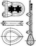
The above mentioned devices for connecting and pairing cables are standardized.
1.4.2. Welding chain
a. Structural characteristics
Welded chain consists of oval links made from round steel bent and then welded by forging or electric welding. The manufacturing material is usually low-carbon steel with low limit, so the tensile strength and load capacity of the chain are low.
b. Basic dimensions
- Chain diameter d x
- Chain step
- Chain width B
- Chain length L: L = t + 2d
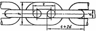
Figure 1.26: Structure of welding chain
c. Classification of welding chains
Based on structure:
- Regular chain.
- Chain with bar.
Based on chain pitch:
- Short chain: t < 3d x
- Long chain: t > 3d x
Based on manufacturing accuracy:
- Chain accuracy: t = ± 0.03d x . and b = ±0.05d x .
- Inaccurate chain: Error of t and B is about ± 0.1d x .
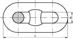
Figure 1.27: Welding chain with crossbar.
d. Characteristics and scope of application
- Easy to bend in all directions (softer than steel cable)
- Simple structure and manufacturing
- Large specific gravity and very sensitive to impacts (noise).
- Susceptible to sudden breakage.
- Chain links are often worn out where they rub.
- Only allows working at slow speed.
- Low tensile strength and low load capacity.
In lifting machines, welded chain is not as widely used as steel wire rope because of its heavy weight and poor reliability.
Usually short link chain is the precision chain used in transmission. Precision chain is used with sprockets with tooth number Z min = 5 with transmission speed not exceeding 0.5 m/s. Non-precision chain is only used with smooth sprockets and drums with transmission speed not exceeding 1 ÷ 5m/s.
Welded chains are suitable for small load lifting mechanisms such as hoists, for transmission in dusty environments where hinge chains cannot be used, or for tying and hanging heavy objects. Welded chains with crossbars are used as anchor chains.
e. Selection method
The chain is mainly subjected to tension, but due to the structure of the chain link, in addition to tension, the chain is also subject to local bending. This stress is difficult to determine, so it is ignored, including the strength of the weld. However, when the chain passes through a drum or pulley, the entire chain link is bent.
Suppose when the chain passes through the pulley, the adjacent links rotate at an angle α. Then the tension force S is divided into two components: (See figure 1.28)