Design of Linear Phase Fir Filter Using Window

exactly the same as the response of the system described by equation (1.28) with a unit pulse signal as the excitation.

1.2. FIR filter design

1.2.1. DESIGN OF LINEAR PHASE FIR FILTER USING WINDOWS

1.2.1.1. Principle:

From the desired frequency response H d (  ) with the corresponding parameters, we take the inverse Fourier transform to get the impulse response h d (  ):

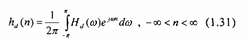
In general, the resulting h d (n) will have infinite length h(n) and be non-causal, which is not feasible in practice. Therefore, the system must be modified to be causal and h(n) must be constrained to the length of h d (n). A simple method is to truncate h d (n) from the value n = M-1 and obtain an FIR filter of length M. This "truncation" is equivalent to multiplying h(n)g by a window function. The window function is defined as follows:

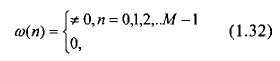
Thus, the impulse response of the FIR filter becomes:

h(n) = h d (n).w(n) (1.33)

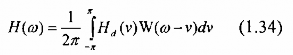
Let W(  ) be the Fourier transform of the window w(n), from the multiplicative property of the Fourier transform, we obtain the frequency response of the filter as follows:

1.2.1.2. Main steps of the window method: Select 4 technical parameters of the digital filter: δ 1 , δ 2 ,  p ,  s . Determine the impulse response of the ideal filter circuit. Select the window type.

Multiply by the window to get the filter impulse response: h d (n) = h(n).w(n). Retest in the frequency domain: H d (  ) = H(  )*W(  ).

If the specifications are not met, we increase M and return to step 2.

1.2.1.3. Rectangular window

Definition: A rectangular window of length M is defined in the time domain.

as follows:

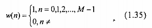
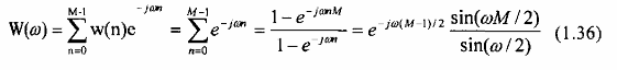
In the odd case, w(n) has a symmetric form with the center of symmetry at n: The Fourier transform of the rectangular window is:

M -1 .

2

This window has an amplitude response of:

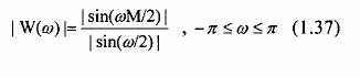
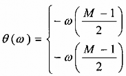
and has a linear phase response:

, when sin (  M)/2  0

, when sin (  M)/2 < 0

1.38

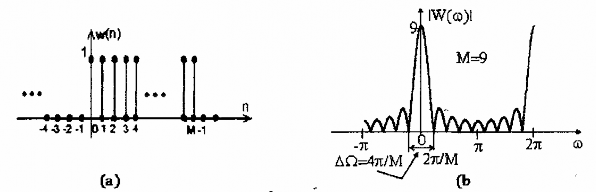
Figure 1.14: (a) Rectangular window with length M = 9

(b) Rectangular window amplitude response

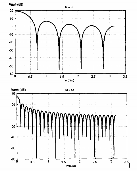
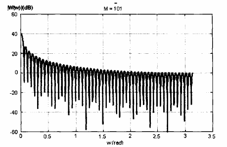
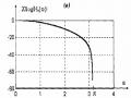
Figure 1.15: Amplitude responses (db) of rectangular windows with M = 9. M = 51 and M-101

Parameters (these parameters are also defined in common for other window types):

- Width of main band DW (calculated as 2 times the frequency range from  = 0 to  p , frequency  p corresponds to zero value of main band), for rectangular window:

DW = 4p/M. (1.39)

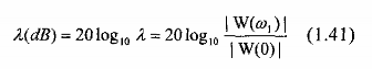
- The ratio between the top of the first lateral cusp and the top of the main cusp, denoted by:

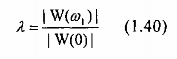
with  1 being the frequency corresponding to the peak of the first side lobe, with a rectangular window w 1 = 3p/M. This parameter is usually calculated as follows:

People also often consider an opposite quantity, which is the ratio of the main cusp tip and the first side cusp tip, denoted by h, we have:

for rectangular windows:

Here are the values ​​of h corresponding to different lengths M:

M = 6 ® h = 4.2426; M = 9 ® h = 4.1000; M = 10 ® h = 4.7014; M = 100 ® h = 4.7106;. ..

and M ® ¥ ~ then h » 4.712. We see that when M > 10 the parameter is almost constant.

Figure 1.14.a shows the rectangular window in the time domain, Figure 1.14.b is the amplitude response of the rectangular window with M = 9. The corresponding parameters are as follows:

DW = 4p/M = 1.3963 rad; 1 = -13.0643dB; h = 4.1000

Figure 1.11 shows the amplitude response of a rectangular window with M being: 9,11 and

101.

Gibbs phenomenon 1

To limit the impulse response length h(n) of the ideal filter, we multiply by the window function w(n). The frequency response of the actual filter is obtained from the convolution (131). For the filter

Ideally, the amplitude response switches abruptly from 1 to 0 (or vice versa) at the cutoff frequency. But for practical filters, due to convolution in the frequency domain, it will cause oscillations in the passband and stopband around the cutoff frequency  c . The generation of these oscillations is called the Gibbs phenomenon.

Example 1.4:

Design a linear phase FIR filter with the following specifications:

δ 1 = 0.01, δ 2 = 0.01,  p =  /4 -  /10 = 0.7226,  =  /4 +  /10 = 0.8482 and  = (  p +  s /2

=  /4.

Prize:

- Choose a rectangular window W(n) with causality and symmetry center at (M- 1)/2.

- To illustrate the Gibbs phenomenon, we choose the frequency response of an ideal low-pass filter, we have:

Taking the inverse Fourier transform, according to equation (1.28), we get the impulse response h(n):

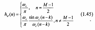
We see that h d (n) has infinite length h(n), is not causal and has a center of symmetry at k in the time domain. If we choose k = (M- 1)/2 then than has a center of symmetry at (M- 1)/2.

Multiplying h(n) by the rectangular window w(n), the filter impulse response becomes causal and has finite length h(n):

h(n) = hd(n) .w(n)

Figure 1.16. Illustration of the impulse response h(n) with M = 61.

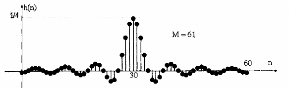
Figure 1.16: Impulse response h(n) sliced ​​from h d (n) and rectangular window M = 61

The frequency response of the designed system is:

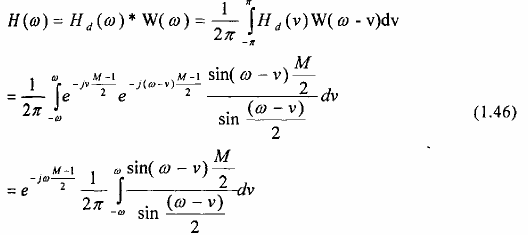
Figure 1.18 plots the amplitude response characteristics of the filter with M = 9, M = 61 and M = 101.

We see that, as M increases, the passband and stopband ripples do not decrease in amplitude and in all three cases, the proposed ripple criterion is not satisfied. However, the transient width is improved (narrowed) as M increases.

To reduce large ripples in both the passband and stopband, we can use window functions that contain a sharp peak and decay gradually to zero instead of abruptly like a rectangular window function.

Some typical window functions commonly used in FIR filter design are shown in Table 1.1 and the shape of some windows is shown in Figure 1.17. These window functions have lower sidelobes than rectangular windows. However, for the same value of M, the width of the main lobe of these window functions is also wider than that of rectangular windows. Therefore, these window functions have the effect of smoothing the frequency response through convolution in the frequency domain, and as a result, the transient band of the FIR filter is wider. To reduce the transient band width, we increase the window length, which results in a larger filter.

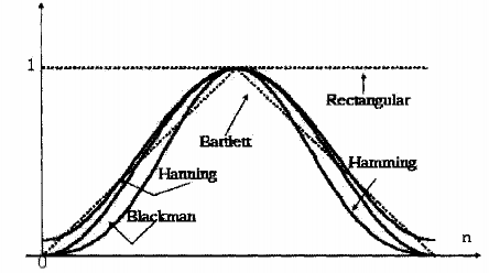
Figure 1.17. The form (envelope) of some window functions in the time domain

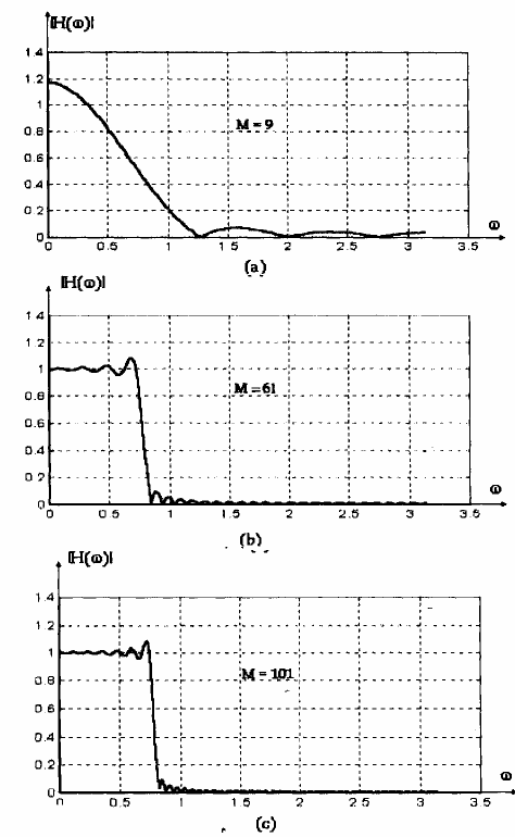
Figure 1.18: Amplitude response of a low-pass filter designed with a rectangular window. (a) M = 9, (b) M = 61, (c) M = 101

Table 1.1. Window functions

Bartlett (triangular)

2n , With 0  n  M  1 M  1 2n 2 - 2n , With 2n < n  M - 1 M  1 M  1
Blackman	w(n) = 0.42 - 0.5cos 2π n -+ 0.08 scos 4π n M  1 M  1
Hamming	w(n) = 0.54 - 0.46 cos 2π n M  1
H(n)ning	w(n) = 1 (1 - cos 2π n ) 2 M  1
Kaiser	I ⎡ M  1 1  ⎛ 2n  1 ⎞ ⎤ ⎢ ⎢ β 2 ⎜ M  1 ⎟ ⎥ ⎥ ⎣ ⎝ ⎠ ⎦ I ⎡ ⎛ M  1 ⎞ ⎤ ⎢ β ⎜2 ⎟ ⎥ ⎣ ⎝ ⎠⎦
Lanczos	⎧ ⎡ 2π ⎛ n  M  1 ⎞ ⎤ ⎫ ⎪ ⎢ ⎜ 2 ⎟ ⎥ ⎪ ⎪ sin ⎢ ⎝ ⎠⎥ ⎪ ⎪ ⎢ M  1 ⎥ ⎪ ⎪⎢⎥⎪ w(n) = ⎨ ⎣ ⎦ ⎛ M  1 ⎞ ⎬ ⎪ ⎜ n  ⎟ ⎪ ⎪ 2π ⎜ 2 ⎟ ⎪ ⎪ ⎜ ⎜ M  1 ⎟ ⎟ ⎪ ⎪ ⎪ ⎝ 2 ⎠ ⎪ ⎪ ⎩⎭
Tukey	1, with n M  1   M  1 , 0 <  < 1 2 2 ⎡ ⎛ n  (1  α) ⎛ M  1 ⎞ ⎞ ⎤ 1 ⎢ ⎜ ⎜ 2 ⎟ ⎟ ⎥ ⎢ 1  cos ⎜⎝⎠ ⎟ ⎥ , 2 ⎢ ⎜ (1  α) ⎛ M  1 ⎞ ⎟ ⎥ ⎢ ⎜ ⎜ 2 ⎟ ⎟ ⎥ ⎣ ⎝ ⎝ ⎠ ⎠ ⎦ With M  1 n  M  1 M  1 2 2 2

Maybe you are interested!

• Amplitude Response Characteristics of a Linear Phase Fir Filter in Example 5.7
• Pulse Characteristics of Linear Phase Fir Digital Filter
• Design of single-phase and three-phase electric meter test bench - 10
• Design and calculation of 3-phase asynchronous motor with Squirrel Cage rotor - 1
• Qos Assurance Methods for Multimedia Communications zt2i3t4l5ee zt2a3gs zt2a3ge zc2o3n4t5e6n7ts low. The EF PHB requires a sufficiently large number of output ports to provide low delay, low loss, and low jitter. EF PHBs can be implemented if the output port's bandwidth is sufficiently large, combined with small buffer sizes and other network resources dedicated to EF packets, to allow the router's service rate for EF packets on an output port to exceed the arrival rate λ of packets at that port. This means that packets with PHB EF are considered with a pre-allocated amount of output bandwidth and a priority that ensures minimum loss, minimum delay and minimum jitter before being put into operation. PHB EF is suitable for channel simulation, leased line simulation, and real-time services such as voice, video without compromising on high loss, delay and jitter values. Figure 2.10 Example of EF installation Figure 2.10 shows an example of an EF PHB implementation. This is a simple priority queue scheduling technique. At the edges of the DS domain, EF packet traffic is prioritized according to the values ​​agreed upon by the SLA. The EF queue in the figure needs to output packets at a rate higher than the packet arrival rate λ. To provide an EF PHB over an end-to-end DS domain, bandwidth at the output ports of the core routers needs to be allocated in advance to ensure the requirement μ > λ. This can be done by a pre-configured provisioning process. In the figure, EF packets are placed in the priority queue (the upper queue). With such a length, the queue can operate with μ > λ. Since EF was primarily used for real-time services such as voice and video, and since real-time services use UDP instead of TCP, RED is generally not suitable for EF queues because applications using UDP will not respond to random packet drop and RED will strip unnecessary packets. 2.2.4.2 Assured Forwarding (AF) PHB PHB AF is defined by RFC 2597. The purpose of PHB AF is to deliver packets reliably and therefore delay and jitter are considered less important than packet loss. PHB AF is suitable for non-real-time services such as applications using TCP. PHB AF first defines four classes: AF1, AF2, AF3, AF4. For each of these AF classes, packets are then classified into three subclasses with three distinct priority levels. Table 2.8 shows the four AF classes and 12 AF subclasses and the DSCP values ​​for the 12 AF subclasses defined by RFC 2597. RFC 2597 also allows for more than three separate priority levels to be added for internal use. However, these separate priority levels will only have internal significance. PHB Class PHB Subclass Package type DSCP AF4 AF41 Short 100010 AF42 Medium 100100 AF43 High 100110 AF3 AF31 Short 011010 AF32 Medium 011100 AF33 High 011110 AF2 AF21 Short 010010 AF22 Medium 010100 AF23 High 010110 AF1 AF11 Short 001010 AF12 Medium 001100 AF13 High 001110 Table 2.8 AF DSCPs The AF PHB ensures that packets are forwarded with a high probability of delivery to the destination within the bounds of the rate agreed upon in an SLA. If AF traffic at an ingress port exceeds the pre-priority rate, which is considered non-compliant or “out of profile”, the excess packets will not be delivered to the destination with the same probability as the packets belonging to the defined traffic or “in profile” packets. When there is network congestion, the out of profile packets are dropped before the in profile packets are dropped. When service levels are defined using AF classes, different quantity and quality between AF classes can be realized by allocating different amounts of bandwidth and buffer space to the four AF classes. Unlike EF, most AF traffic is non-real-time traffic using TCP, and the RED queue management strategy is an AQM (Adaptive Queue Management) strategy suitable for use in AF PHBs. The four AF PHB layers can be implemented as four separate queues. The output port bandwidth is divided into four AF queues. For each AF queue, packets are marked with three “colors” corresponding to three separate priority levels. In addition to the 32 DSCP 1 groups defined in Table 2.8, 21 DSCPs have been standardized as follows: one for PHB EF, 12 for PHB AF, and 8 for CSCP. There are 11 DSCP 1 groups still available for other standards. 2.2.5.Example of Differentiated Services We will look at an example of the Differentiated Service model and mechanism of operation. The architecture of Differentiated Service consists of two basic sets of functions: Edge functions: include packet classification and traffic conditioning. At the inbound edge of the network, incoming packets are marked. In particular, the DS field in the packet header is set to a certain value. For example, in Figure 2.12, packets sent from H1 to H3 are marked at R1, while packets from H2 to H4 are marked at R2. The labels on the received packets identify the service class to which they belong. Different traffic classes receive different services in the core network. The RFC definition uses the term behavior aggregate rather than the term traffic class. After being marked, a packet can be forwarded immediately into the network, delayed for a period of time before being forwarded, or dropped. We will see that there are many factors that affect how a packet is marked, and whether it is forwarded immediately, delayed, or dropped. Figure 2.12 DiffServ Example Core functionality: When a DS-marked packet arrives at a Diffservcapable router, the packet is forwarded to the next router based on Per-hop behavior is associated with packet classes. Per-hop behavior affects router buffers and the bandwidth shared between competing classes. An important principle of the Differentiated Service architecture is that a router's per-hop behavior is based only on the packet's marking or the class to which it belongs. Therefore, if packets sent from H1 to H3 as shown in the figure receive the same marking as packets from H2 to H4, then the network routers treat the packets exactly the same, regardless of whether the packet originated from H1 or H2. For example, R3 does not distinguish between packets from h1 and H2 when forwarding packets to R4. Therefore, the Differentiated Service architecture avoids the need to maintain router state about separate source-destination pairs, which is important for network scalability. Chapter Conclusion Chapter 2 has presented and clarified two main models of deploying and installing quality of service in IP networks. While the traditional best-effort model has many disadvantages, later models such as IntServ and DiffServ have partly solved the problems that best-effort could not solve. IntServ follows the direction of ensuring quality of service for each separate flow, it is built similar to the circuit switching model with the use of the RSVP resource reservation protocol. IntSer is suitable for services that require fixed bandwidth that is not shared such as VoIP services, multicast TV services. However, IntSer has disadvantages such as using a lot of network resources, low scalability and lack of flexibility. DiffServ was born with the idea of ​​solving the disadvantages of the IntServ model. DiffServ follows the direction of ensuring quality based on the principle of hop-by-hop behavior based on the priority of marked packets. The policy for different types of traffic is decided by the administrator and can be changed according to reality, so it is very flexible. DiffServ makes better use of network resources, avoiding idle bandwidth and processing capacity on routers. In addition, the DifServ model can be deployed on many independent domains, so the ability to expand the network becomes easy. Chapter 3: METHODS TO ENSURE QoS FOR MULTIMEDIA COMMUNICATIONS In packet-switched networks, different packet flows often have to share the transmission medium all the way to the destination station. To ensure the fair and efficient allocation of bandwidth to flows, appropriate serving mechanisms are required at network nodes, especially at gateways or routers, where many different data flows often pass through. The scheduler is responsible for serving packets of the selected flow and deciding which packet will be served next. Here, a flow is understood as a set of packets belonging to the same priority class, or originating from the same source, or having the same source and destination addresses, etc. In normal state when there is no congestion, packets will be sent as soon as they are delivered. In case of congestion, if QoS assurance methods are not applied, prolonged congestion can cause packet drops, affecting service quality. In some cases, congestion is prolonged and widespread in the network, which can easily lead to the network being "frozen", or many packets being dropped, seriously affecting service quality. Therefore, in this chapter, in sections 3.2 and 3.3, we introduce some typical network traffic load monitoring techniques to predict and prevent congestion before it occurs through the measure of dropping (removing) packets early when there are signs of impending congestion. 3.1. DropTail method DropTail is a simple, traditional queue management method based on FIFO mechanism. All incoming packets are placed in the queue, when the queue is full, the later packets are dropped. Due to its simplicity and ease of implementation, DropTail has been used for many years on Internet router systems. However, this algorithm has the following disadvantages: − Cannot avoid the phenomenon of “Lock out”: Occurs when 1 or several traffic streams monopolize the queue, making packets of other connections unable to pass through the router. This phenomenon greatly affects reliable transmission protocols such as TCP. According to the anti-congestion algorithm, when locked out, the TCP connection stream will reduce the window size and reduce the packet transmission speed exponentially. − Can cause Global Synchronization: This is the result of a severe “Lock out” phenomenon. Some neighboring routers have their queues monopolized by a number of connections, causing a series of other TCP connections to be unable to pass through and simultaneously reducing the transmission speed. After those monopolized connections are temporarily suspended, Once the queue is cleared, it takes a considerable amount of time for TCP connections to return to their original speed. − Full Queue phenomenon: Data transmitted on the Internet often has an explosion, packets arriving at the router are often in clusters rather than in turn. Therefore, the operating mechanism of DropTail makes the queue easily full for a long period of time, leading to the average delay time of large packets. To avoid this phenomenon, with DropTail, the only way is to increase the router's buffer, this method is very expensive and ineffective. − No QoS guarantee: With the DropTail mechanism, there is no way to prioritize important packets to be transmitted through the router earlier when all are in the queue. Meanwhile, with multimedia communication, ensuring connection and stable speed is extremely important and the DropTail algorithm cannot satisfy. The problem of choosing the buffer size of the routers in the network is to “absorb” short bursts of traffic without causing too much queuing delay. This is necessary in bursty data transmission. The queue size determines the size of the packet bursts (traffic spikes) that we want to be able to transmit without being dropped at the routers. In IP-based application networks, packet dropping is an important mechanism for indirectly reporting congestion to end stations. A solution that prevents router queues from filling up while reducing the packet drop rate is called dynamic queue management. 3.2. Random elimination method – RED 3.2.1 Overview RED (Random Early Detection of congestion; Random Early Drop) is one of the first AQM algorithms proposed in 1993 by Sally Floyd and Van Jacobson, two scientists at the Lawrence Berkeley Laboratory of the University of California, USA. Due to its outstanding advantages compared to previous queue management algorithms, RED has been widely installed and deployed on the Internet. The most fundamental point of their work is that the most effective place to detect congestion and react to it is at the gateway or router. Source entities (senders) can also do this by estimating end-to-end delay, throughput variability, or the rate of packet retransmissions due to drop. However, the sender and receiver view of a particular connection cannot tell which gateways on the network are congested, and cannot distinguish between propagation delay and queuing delay. Only the gateway has a true view of the state of the queue, the link share of the connections passing through it at any given time, and the quality of service requirements of the traffic flows. The RED gateway monitors the average queue length, which detects early signs of impending congestion (average queue length exceeding a predetermined threshold) and reacts appropriately in one of two ways: − Drop incoming packets with a certain probability, to indirectly inform the source of congestion, the source needs to reduce the transmission rate to keep the queue from filling up, maintaining the ability to absorb incoming traffic spikes. − Mark “congestion” with a certain probability in the ECN field in the header of TCP packets to notify the source (the receiving entity will copy this bit into the acknowledgement packet). Figure 3. 1 RED algorithm The main goal of RED is to avoid congestion by keeping the average queue size within a sufficiently small and stable region, which also means keeping the queuing delay sufficiently small and stable. Achieving this goal also helps: avoid global synchronization, not resist bursty traffic flows (i.e. flows with low average throughput but high volatility), and maintain an upper bound on the average queue size even in the absence of cooperation from transport layer protocols. To achieve the above goals, RED gateways must do the following: − The first is to detect congestion early and react appropriately to keep the average queue size small enough to keep the network operating in the low latency, high throughput region, while still allowing the queue size to fluctuate within a certain range to absorb short-term fluctuations. As discussed above, the gateway is the most appropriate place to detect congestion and is also the most appropriate place to decide which specific connection to report congestion to. − The second thing is to notify the source of congestion. This is done by marking and notifying the source to reduce traffic. Normally the RED gateway will randomly drop packets. However, if congestion If congestion is detected before the queue is full, it should be combined with packet marking to signal congestion. The RED gateway has two options: drop or mark; where marking is done by marking the ECN field of the packet with a certain probability, to signal the source to reduce the traffic entering the network. − An important goal that RED gateways need to achieve is to avoid global synchronization and not to resist traffic flows that have a sudden characteristic. Global synchronization occurs when all connections simultaneously reduce their transmission window size, leading to a severe drop in throughput at the same time. On the other hand, Drop Tail or Random Drop strategies are very sensitive to sudden flows; that is, the gateway queue will often overflow when packets from these flows arrive. To avoid these two phenomena, gateways can use special algorithms to detect congestion and decide which connections will be notified of congestion at the gateway. The RED gateway randomly selects incoming packets to mark; with this method, the probability of marking a packet from a particular connection is proportional to the connection's shared bandwidth at the gateway. − Another goal is to control the average queue size even without cooperation from the source entities. This can be done by dropping packets when the average size exceeds an upper threshold (instead of marking it). This approach is necessary in cases where most connections have transmission times that are less than the round-trip time, or where the source entities are not able to reduce traffic in response to marking or dropping packets (such as UDP flows). 3.2.2 Algorithm This section describes the algorithm for RED gateways. RED gateways calculate the average queue size using a low-pass filter. This average queue size is compared with two thresholds: minth and maxth. When the average queue size is less than the lower threshold, no incoming packets are marked or dropped; when the average queue size is greater than the upper threshold, all incoming packets are dropped. When the average queue size is between minth and maxth, each incoming packet is marked or dropped with a probability pa, where pa is a function of the average queue size avg; the probability of marking or dropping a packet for a particular connection is proportional to the bandwidth share of that connection at the gateway. The general algorithm for a RED gateway is described as follows: [5] For each packet arrival Caculate the average queue size avg If minth ≤ avg < maxth div.maincontent .s1 { color: black; font-family:"Times New Roman", serif; font-style: normal; font-weight: normal; text-decoration: none; font-size: 15pt; } div.maincontent .s2 { color: black; font-family:"Times New Roman", serif; font-style: normal; font-weight: bold; text-decoration: none; font-size: 15pt; } div.maincontent .p { color: black; font-family:"Times New Roman", serif; font-style: normal; font-weight: normal; text-decoration: none; font-size: 14pt; margin:0pt; } div.maincontent p { color: black; font-family:"Times New Roman", serif; font-style: normal; font-weight: normal; text-decoration: none; font-size: 14pt; margin:0pt; } div.maincontent .s3 { color: black; font-family:"Times New Roman", serif; font-style: normal; font-weight: bold; text-decoration: none; font-size: 14pt; } div.maincontent .s4 { color: black; font-family:"Times New Roman", serif; font-style: normal; font-weight: normal; text-decoration: none; font-size: 14pt; } div.maincontent .s5 { color: black; font-family:"Times New Roman", serif; font-style: italic; font-weight: normal; text-decoration: none; font-size: 14pt; } div.maincontent .s6 { color: black; font-family:"Times New Roman", serif; font-style: italic; font-weight: bold; text-decoration: none; font-size: 14pt; } div.maincontent .s7 { color: black; font-family:Wingdings; font-style: normal; font-weight: normal; text-decoration: none; font-size: 14pt; } div.maincontent .s8 { color: black; font-family:Arial, sans-serif; font-style: italic; font-weight: bold; text-decoration: none; font-size: 15pt; } div.maincontent .s9 { color: black; font-family:"Times New Roman", serif; font-style: normal; font-weight: bold; text-decoration: none; font-size: 14pt; } div.maincontent .s10 { color: black; font-family:"Times New Roman", serif; font-style: normal; font-weight: normal; text-decoration: none; font-size: 9pt; vertical-align: 6pt; } div.maincontent .s11 { color: black; font-family:"Times New Roman", serif; font-style: normal; font-weight: normal; text-decoration: none; font-size: 13pt; } div.maincontent .s12 { color: black; font-family:"Times New Roman", serif; font-style: normal; font-weight: normal; text-decoration: none; font-size: 10pt; } div.maincontent .s13 { color: black; font-family:"Times New Roman", serif; font-style: normal; font-weight: normal; text-d

Note: The Kaiser window is a near-optimal window, which is formed from the first-order non-zero Bessel function I 0 (x). In the Kaiser window definition formula (Table