The mathematical expectation of a variable is a value in a population determined by the following formula:
Discrete random variable:
Maybe you are interested!
-

 Perfecting the Audit Method to Determine Enterprise Value
 -
 Building a method for training high school teachers under contract between Ho Chi Minh City University of Education and some southern provinces - 11
 -
 Research on the treatment of seafood wastewater by electrocoagulation method combined with USBF - 19 tank
 -
 Revenue Forecast of Nam Viet Corporation 2014 Using Brown Method
 -
 Equivalent Annual Payment Method
(with p i

n
E ( X ) ∑ x ip i
i 1
is the probability that the random variable X takes on the value
x i )
(1.23)
Continuous random variable with probability density function f ( x ) :
E ( x )
∫xf ( x ) dx
(1.24)
The mathematical expectation value of a random variable will give the central value of that variable. However, in statistics and data analysis, having the entire population is unlikely to happen, so the estimate for the mathematical expectation is the sample mean instead. The sample mean is usually calculated using the arithmetic mean formula as follows:
n
1
X ∑ X i
(1.25)
n i 1
Variance – Standard Error
When we have all the information about the population to be studied, we have:
The overall variance of variable X is:
2 var( X ) E ( X E ( X )) 2
(1.26)
Standard deviation:
se ( X )
(1.27)
var( X )
When we only observe the whole through a sample of size n
Sample variance:
S 2
1
n 1
n
∑
i 1
( X 1
X ) 2
(1.28)
1∑ n(
n 1
X X
i
) 2
i 1
Sample standard deviation: S (1.29)
The meaning of variance and standard deviation in economic data analysis:
This characteristic reflects the degree of dispersion of the values of the oscillator variable.
around its mean value, this feature can also be used to detect the homogeneity of data between different groups of subjects of interest.
Dispersion range
The range is the distance from the smallest value to the largest value in a series of observations.
Coefficient of variation
The ratio of the standard deviation to the mean of a random variable:
X
E ( X )
CV
100%
If
E ( X ) 0
(1.30)
The smaller the value of the coefficient of variation, the greater the homogeneity of the data series and vice versa. In addition, this coefficient is also used to compare the dispersion of two variables whose mathematical expectation and standard deviation are different.
Skewness coefficient
The degree of symmetry in the distribution of a variable is expressed through the value of the asymmetry coefficient:
3
(1.31)
in there
3
3 3
3 E [ X E ( X )] and
3
is the cube of the standard deviation. For the
close to the sample, this coefficient is calculated as follows:
∑
1
n
( X i
n
X ) 3
S i 1 3 S3
(1.32)
where S is the sample standard deviation of variable X.
Depends on the value of 3 , the analyst can draw the following conclusions:
3 > 0, the distribution of the variable is asymmetrical and the graph will be more to the right.
3 = 0, the distribution is symmetrical
3 < 0, the distribution of the variable is asymmetrical and the graph will be more to the left.
Kurtosis
The kurtosis coefficient gives additional information about the variance value. It is calculated by the formula:
4
(1.33)
in there
4
4 4
4 E [ X E ( X )] and
4
is the square of the variance. For the
close to the sample, this coefficient is calculated as follows:
X
1∑ n (
X ) 4
i
S 4
n i 1
S4
(1.34)
where S is the sample standard deviation of variable X.
When the distribution is centered at normal then the median is higher then 4 3 and vice versa.
4 3 , and the set
Two distributional parameters will be used to test the final hypothesis of the OLS method mentioned in the following section.
Correlation coefficient
The correlation coefficient between two variables is calculated according to the following formula:
r ( X , Y )
∑ ( X i X )( Y i Y )
(1.35)
∑ ( X i X ) ∑ ( Y
2
i
Y ) 2
The value of the correlation coefficient indicates how strong the linear relationship between the variables is and also indicates the direction of the relationship between the variables.
1.3.2 . Estimation methods used in econometric model building
The method used to estimate the parameters of the model is the very popular OLS (Odinary Less Square) method, the ordinary least squares method. This is an estimation method independently proposed by two mathematicians Carl Federic Guass (German) and Laplace (French) [35].
1.3.2.1.Content of OLS method
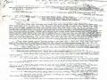
From the perspective of econometrics, the movement of an economic variable is subject to two influences: the first influence is due to factors that systematically affect it (this can be understood as the influence of independent variables in the econometric model) and the second part is other random factors that have an unsystematic influence on the dependent variable (this component is called the error or random factor of the model). When using sample data to estimate the parameters of an econometric model, random errors are represented by the values of the residuals in the sample regression function.
C ¸ cquans ¸ tc đ am Europa
® - I mean
European Union
C ¸ cph Ç nd −
Figure 1.3 . Values of residuals in sample regression function
It can be seen that the smaller the absolute value of the residuals, the more accurate the estimates. Therefore, the estimation criterion of the OLS method is based on the sum of squares of the residuals reaching the minimum value.
1.3.2.2 . Assumptions of the OLS method
The OLS method makes several assumptions to ensure the accuracy of the estimates:
Assumption 1 : Random errors have an expectation of 0: E(U i ) ( i ) . In practice, this assumption only makes sense in theory because when estimating by the OLS method, the image of random errors in the sample is the residuals that have an expectation = 0.
Assumption 2 : There is no correlation between random errors Covariance (U i , U j ) = 0 ( i j )
Assumption 3 : The random errors are homogeneous Variance ( U i ) = 2- ( i )
Hypothesis 4 : There is no linear relationship between independent variables. Hypothesis 5 : Random error U i has a normal distribution U i ~ N ( 0, 2 ) Hypothesis 6 : The model has the correct form and is not missing variables .
The above assumptions will be tested in turn after conducting the estimation.
R2 coefficient measures the goodness of fit of the sample regression function
RSS =
∑ ( Y Y ) 2 ∑ e 2
(1.36)
n
n
i 1 1 i 1 1
RSS (Residual Sum of Square) is the sum of squares of all the differences between the observed Y values and the values obtained from the regression function.
TSS = ESS + RSS
TSS is the sum of squares of all the deviations between the observed values Y i and their mean values.
TSS =
∑ y 2∑ ( Y
Y ) 2
(1.37)
n
n
i 1 i i 1i
2
ESS is the sum of the squares of all the deviations between the values of the dependent variable Y obtained from the sample regression function and their mean values. This part measures the accuracy of the regression function.
ESS = ∑ ( Y
n
1
i 1
Y ) 2
∑ y 2
n
i 1 i
β 2
∑ x2
n
i 1i
(1.38)
1 = ESS
RSS
∑ ( Y
Y ) 2 2
(1.39)
n
n
e
i
∑
i
i 1
n
i 1
n
put
TSS
TSS
∑ ( Y
i
i 1
Y ) 2
∑ ( Y
i
i 1
Y ) 2
n
∑ ( Y
2
i
Y ) 2
ESS
RSS
(1.40)
r i 1
n
1
i
∑ ( Y
i 1
Y ) 2
TSS
TSS
After some transformations, we can calculate:
r 2
2
x
y
∑ n
i 1 ii
n
n
(1.41)
∑ x 2 ∑ y 2
i 1
i i 1 i
From the definition of r 2 , we see that r 2 measures the percentage of change in the total deviation of Y from its mean value that is explained by the model. Therefore, r 2 measures the goodness of fit of the regression function. It is easy to see that 0 =< r 2 <= 1.
1.3.3 . Some econometric models applied in building the capital structure of enterprises in the world
1.3.3.1 . Research model on the relationship between asset structure and capital structure
Federick H. deB. Harris, a professor at Wake Forest University, Winston Salem State, USA, proposed a model to study the relationship between asset structure, revenue coverage and capital structure.
Investment and financing are always interrelated. To resolve the conflicting debates about the relationship between investment - debt use and growth, it is necessary to build an empirical model between industry structure and financial structure to verify the relationship between marginal profit, revenue coverage, debt use and risk. Using data on expected cumulative losses over discontinuous periods to measure the liquidation value of assets, in the investment activities of enterprises, the verification results will be used to support the study of the relationship between investment and debt use, between the growth rate of debt and the growth rate of enterprises, the level of equity financing for growth and the level of debt financing for specific assets. These evidences would refute the theory of the impact of transaction costs on capital structure in the study of Fortune 500 companies [ 52 ] .
Capital structure model
LTD/TA = f(TA/SAL, GPCM, YEILD, beta, AS/SAL, ExQ, NB) (1.42)
In there:
LTD/TA: Long-term debt to total assets
GPCM = price - marginal cost = (revenue - direct cost)/total revenue Yield: yield to maturity of corporate bonds, 1 year
AS/SAL: asset specificity ExG: expected earnings growth rate
NB: number of new products launched in a year
The capital structure model is interpreted by a reduced model of the ratio of Long-term Debt to Total Assets (LTD/TA). The expected revenue coverage TA/SAL increases in the same direction as long-term debt in the capital structure of the enterprise, while the expected profit GPCM fluctuates in the opposite direction with the debt ratio. These relationships are explained at the 99% significance level (o = 0.01). Similarly, in Baker's study in 1973, enterprises with high marginal profits tend to increase the use of internal financing rather than debt. In the TSLS method (2-stage squared), higher absolute marginal profits ABSOLU (measure of cost per unit of debt) will reduce the use of debt, reducing LTD/TA. With low costs, equity, as expected, will replace the use of debt in the cross-sectional analysis model. The cost of equity measure, which is a factor that has a significant positive relationship with debt usage in the two-stage squared (TSLS) model.
Consistent with the studies of Harris (1984) and Stulz (1990), the expected profit growth rate (EXANTEG) does not have any effect on the debt ratio [52]. In these studies, it is shown that only current and past profit rates are factors affecting the use of debt, not the future profit growth rate.
Williamson's theory of the impact of transaction costs on the use of debt has been rejected because the test results show that asset structure
has a significant positive relationship with the use of debt, while Williamson's study suggests that increasing asset structure leads to increasing use of equity.
Systemic risk model
õ = f (RM, RSQQ, GPCM, LTD/TA, TA, CF) (1.43)
+ - + + - +
In there:
õ: statistical beta coefficient value calculated by average month from 1967 to
1971
RM: correlation coefficient between market return and company return
monthly
RSQQ: RsquareQ: R 2 method for estimating industry-wide output over time series
CF: fixed cost = investment cost of machinery and equipment + inventory In the TSLS method (two-stage square) forecasting about
The beta equation shows that systematic risk increases as the firm's output increases with a given monthly correlation coefficient between the firm's return and the market (RM). Furthermore, if the book value (TA) of assets increases sufficiently to match the variance of the market value, the beta decreases. A shorthand measure of the debt ratio, Long-term debt to total assets (LTD/TA), has been predicted to have a relationship with risk, with more debt used leading to increased risk. Both fixed costs (reflecting the technological characteristics of the industry) and marginal revenue have no significant effect on beta in the TSLQ model.
1.3.3.2 . Research model of tax impact on capital structure
Reinte Gropp, a prominent economist at the European Central Bank, proposed a research model that incorporated various German government taxes in 2002. The model also included business taxes.