Summary of Factors and Observed Variables After Efa

4.3.3 Summary of factors and observed variables after EFA

In summary, after the author conducted EFA analysis for 5 independent variables and 1 dependent variable, the results of the number of factors and variables retained for the study were 5 independent variables (including 21 observed variables, including 6 observed variables proposed by the author, 15 variables inherited by the author from the 2006 adjusted HEdPERF scale) and 1 dependent factor (including 3 observed variables inherited by the author from Dang Thi Ho Thuy 2018) presented in the following table (see Appendix 11 for details).

Table 4.6: Summary of factors and observed variables after EFA

STT

Factor name	Observation variable	Number of observed variables
1	Academic	Aca1, Aca2, Aca4	3
2	Non-academic	N – Aca1, N- Aca2, N- Aca3, N-Aca4	4
3	Reputation	Rep3, Rep4, Rep5	3
4	Approach	Acc1, Acc2, Acc3, Acc4, Acc5, Acc6, Acc7	7
5	Training program	Pro2, Pro3, Pro4, Pro5	4
6	Student satisfaction	Sat1, Sat2, Sat3	3
Total			24

Maybe you are interested!

(Source: Author's synthesis)

4.4 Multiple regression analysis

4.4.1 Test the correlation between independent variables and dependent variables

Before regression analysis, we need to consider the correlation between the independent variable and the dependent variable (using Pearson correlation). If any independent variable has a strong correlation with the dependent variable, meaning Sig. (2-tailed) < 0.05, it will be included in the regression because it is statistically significant, but any variable with Sig. (2-tailed) > 0.05 will not.

entered into the regression because it was not statistically significant. The results of the Pearson correlation test between the independent and dependent variables are shown in Appendix 12.

Table 4.7: Correlation results between independent variables and dependent variables

Factor

N	Student satisfaction with training service quality create
Academic	Correlate Pearson	208	0.742 **
	Sig. (2-tailed)		0.000
Non-academic	Correlate Pearson	208	0.735 **
	Sig. (2-tailed)		0.000
Reputation	Correlate Pearson	208	0.496 **
	Sig. (2-tailed)		0.000
Approach	Correlate Pearson	208	0.523 **
	Sig. (2-tailed)		0.000
Training program	Correlate Pearson	208	0.698 **
	Sig. (2-tailed)		0.000

(Source: Author processed data using SPSS software)

From the above results, we can see that the dependent variable has a linear correlation with 5 independent variables at the significance level of 0.000 < 0.05 and the correlation coefficient between the dependent variable "Satisfaction" and the independent variable "Academic" is 0.742; the correlation coefficient between the dependent variable and the independent variable "Non-academic" is 0.735; the correlation coefficient between the dependent variable and the independent variable "Reputation" is 0.496; the correlation coefficient between the dependent variable and the independent variable "Access" is 0.523; the correlation coefficient between the variable

dependent variable with the independent variable “Training Program” is 0.698. Thus, these factors are used to enter into linear regression analysis in the next section.

4.4.2 Linear regression analysis

Table 4.8: Results of the first regression coefficient

Model

Regression coefficient not standardized		Regression coefficient standardized	t (t-Test)	Significance level Sig.
B	Error standard	Beta	t (t-Test)	Significance level Sig.
1	Constant	-0.162	0.172		-0.944	0.346
	Academic	0.357	0.038	0.390	9,304	0.000
	Non-academic	0.310	0.039	0.343	7,920	0.000
	Reputation	0.064	0.040	0.067	1,593	0.113
	Approach	0.071	0.047	0.063	1,492	0.137
	Programme train	0.233	0.046	0.239	5,048	0.000

(Source: The author processed data using SPSS software) The first regression analysis results showed that the correlation coefficient value was 0.880 > 0.5; the coefficient of determination R 2 adjusted = 0.769 at the significance level of 0.000 < 0.05, so the adjusted R 2 is statistically significant or in other words, the 5 independent variables included in the regression model affected 76.9% of the change in the dependent variable, the remaining 23.1% was due to variables outside the model and random errors. In addition, the Durbin-Watson index = 1.940 is within the allowable range from 1 to 3, so there is no autocorrelation phenomenon. However, looking at Table 4.8 to examine the reliability of the independent variables in the model, we see that there are 2 independent variables, "Reputation" and "Approach", with Sig. (significance level) are 0.113 and 0.137 > 0.05 (5% confidence level), respectively. Therefore, these two independent variables will be eliminated in the next regression analysis, but the independent variable with the larger value will be eliminated first. Therefore, in this case, the variable "Approach" will be eliminated first and the author will analyze the regression model for the second time. After eliminating the variable "approach" to analyze the regression model for the next time, the result

The results show that all parameters such as VIF, Tolorence, t stat and Sig. are satisfied (Appendix 12). The results of linear regression analysis are shown as follows:

Table 4.9: Results of the second regression coefficient

Model

Unstandardized regression coefficients		Standardized regression coefficient	t (t-Test)	Significance level Sig.
B	Standard error	Beta	t (t-Test)	Significance level Sig.
1	Constant	-0.47	0.154		-0.308	0.758
	Academic	0.368	0.038	0.402	9,725	0.000
	Non-academic	0.310	0.039	0.343	7,885	0.000
	Reputation	0.081	0.038	0.085	2,115	0.036
	Programme train	0.252	0.045	0.258	5,646	0.000

(Source: Author processed data using SPSS software)

Table 4.10: Model synthesis coefficients

Tissue

image

R 2

R 2 effect

adjust

Standard error

of estimate

Durbin-

Watson

0.879

0.773

0.768

0.30021

1,935

(Source: Author processed data using SPSS software)

The results show that the correlation coefficient value is 0.879 > 0.5; this is a suitable model to use to evaluate the relationship between the dependent variable and the independent variables. In addition, the adjusted coefficient of determination R2 value is 0.768, which means that the constructed linear regression model fits the data 76.8%. In other words, 76.8% of the satisfaction with the training quality of students of the Faculty of Tourism, HUFI is explained by the independent variables of this regression model, the rest is due to errors and other factors. This difference can also be explained by the fact that the research model does not focus on the values and personal characteristics of students such as psychology, personality, etc. Therefore, the observed variable values in the study can only explain 76.8% of the satisfaction with the training quality of students of the Faculty of Tourism, HUFI. And this is also one of the limitations of the topic and will be developed in future studies.

Table 4.11: Testing the suitability of the overall linear regression model

ANOVA a

Model		Total average direction	Df	Mean square jar	F	Sig.
1	Regression	62,130	4	15,533	172,346	0.000 b
	Balance	18,295	203	0.090
	Total	80,425	207

(Source: Author processed data using SPSS software)

The nature of the population is very large, so it is very time-consuming and costly to collect the population, so the author chooses the sample size in the population to infer the population. Therefore, when performing the test in Table 4.11, the author wants his sample size to meet the criteria to be able to infer the research population. The F test is used to evaluate the suitability of this linear regression model to generalize and apply to the population or not? Specifically in this case, the Sig. value of the F test is 0.000 < 0.05, so the linear regression model built is suitable for the population. Thus, finally in the analysis of the linear regression model, we have the following table of results:

Table 4.12: Regression coefficient results and multicollinearity statistics

Model

Unstandardized coefficient		Coefficient standardize	t	Significance level Sig.	Multicollinearity statistics
B	Error standard	Beta	t	Significance level Sig.	Tolerance	VIF
1	Constant	-0.047	0.154		-0.308	0.758
	Academic	0.368	0.038	0.402	9,725	0.000	0.656	1,525
	Non-academic	0.310	0.039	0.343	7,885	0.000	0.594	1,685
	Reputation	0.081	0.038	0.085	2,115	0.036	0.696	1,437
	Programme train	0.252	0.045	0.258	5,646	0.000	0.535	1,868

(Source: Author processed data using SPSS software)

Based on the results of Table 4.12, the author finds that firstly, the Sig. value of the t-test for each independent variable is less than 0.05, which means that the independent variables included in the model are all significant. Second, the standardized regression coefficient, the factors that have

The standardized regression weights have positive signs, meaning that these independent variables have a positive impact on the dependent variable. Finally, all VIF coefficients are < 2, so there is no multicollinearity (Nguyen Dinh Tho, 2011).

From the above results, the standardized linear regression equation is constructed as follows:

Satisfaction with training services of students of Faculty of Tourism, HUFI = 0.402*Academic + 0.343*Non-academic + 0.085*Reputation + 0.258* Training program.

Through the standardized multivariate regression equation above, we can see that there are 4 factors including Academic, Non-academic, Reputation and Training Program that all have a proportional impact on the satisfaction with the training service quality of students of the Faculty of Tourism, HUFI. In addition, the higher the Beta value of these variables, the greater the impact on the satisfaction with the training service quality of students of the Faculty of Tourism, HUFI. The author arranges in order the level of influence of each independent variable on the dependent variable from strongest to weakest as follows:

- First, “Academics” has the most influence with coefficient β = 0.402.

- Second is “Non-academic” which has the next influence with coefficient β = 0.343.

- The third is “Training Program” with coefficient β = 0.258.

- Finally, “Reputation” has the weakest impact with coefficient β = 0.085.

4.4.3 Detecting violations of necessary assumptions in linear regression

- Assume the residuals are normally distributed

To detect violations of the normal distribution assumption of the residuals, we will use two drawing tools of SPSS software: Histogram and PP plot.

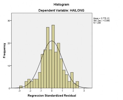
Figure 4.1: Histogram of standardized residual scatter

(Source: Results of author's survey data processing)

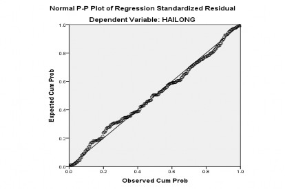
Figure 4.2: PP Plot of standardized regression residuals

(Source: Results of author's survey data processing)

Figure 4.1 shows that almost all the frequency columns are in the bell-shaped graph with mean error close to 0 (Mean value = 3.77E-15 and standard deviation Std.Dev. = 0.990). In addition, Figure 4.2 shows that almost all the observations are distributed around the sample linear regression line. Therefore, the study of

We have a roughly normal distribution, that is, the assumption of normal distribution of the residuals is not violated.

- Assume linearity and constant error variance

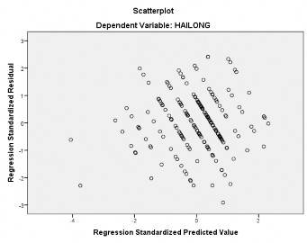
Figure 4.3: Scatter plot of residuals and predicted values of linear regression model

(Source: Results of author's survey data processing)

Figure 4.3 shows that a total of 208 observations are clustered into straight lines, with very few observations falling outside, so it can be concluded that the relationship between the independent and dependent variables in this study is linear.

4.4.4 Testing the hypotheses of the formal research model

Based on the results of Table 4.12, the author concludes that there are 4 hypotheses including H1, H2, H3 and H5 with Sig values all less than 0.05 and the β coefficients are all positive, so these hypotheses are all accepted, as well as the factors all have a positive impact on student satisfaction with the training service quality at the Faculty of Tourism, HUFI with a confidence level of 95%; however, hypothesis H4 is rejected or not accepted because it has Sig > 0.05. Hypothesis H4 states that access has a positive impact on student satisfaction with the training service quality at the Faculty of Tourism, HUFI. Finally, through analysis and evaluation, the research model is adjusted as follows:

Comment