Table 4. 3. Summary of EFA analysis of dependent variables
STT
Variable | Factor | |
1 | ||
1 | BE1 | 0.712 |
2 | BE2 | 0.799 |
3 | BE3 | 0.857 |
4 | BE4 | 0.876 |
Cronbach's Alpha | 0.856 | |
KMO | 0.742 | |
Bartlett (Sig.) | 0.000 | |
Total variance extracted (%) | 66.165 % | |
Maybe you are interested!
-
 EFA Analysis Results for Dependent Variable Group (Preliminary Quantitative Research Phase)
 -
 Summary Table of Exploratory Factor Analysis Results Efa
 -
 Rotated Factor Matrix Efa of Dependent Variable
 -
 Identify Rating Levels and Rating Scales
zt2i3t4l5ee
zt2a3gstourism,quan lan,quang ninh,ecology,ecotourism,minh chau,van don,geography,geographical basis,tourism development,science
zt2a3ge
zc2o3n4t5e6n7ts
of the islanders. Therefore, this indicator will be divided into two sub-indicators:
a1. Natural tourism attractiveness a2. Cultural tourism attractiveness
b. Tourist capacity
The two island communes in Quan Lan have different capacities to receive tourists. Minh Chau Commune is home to many standard hotels and resorts, attracting high-income domestic and international tourists. Meanwhile, Quan Lan Commune has many motels mainly built and operated by local people, so the scale and quality are not high, and will be suitable for ordinary tourists such as students.
c. Time of exploitation of Quan Lan Island Commune:
Quan Lan tourism is seasonal due to weather and climate conditions and festivals only take place on certain days of the year, specifically in spring. In Quan Lan commune, the period from April to June and from September to November is considered the best time to visit Quan Lan because the cultural tourism activities are mainly associated with festivals taking place during this time.
Minh Chau island commune:
Tourism exploitation time is all year round, because this is a place with a number of tourist attractions with diverse ecosystems such as Bai Tu Long National Park Research Center, Tram forest, Turtle Laying Beach, so besides coming to the beach for tourism and vacation in the summer, Minh Chau will attract research groups to come for tourism combined with research at other times of the year.
d. Sustainability
The sustainability of ecotourism sites in Quan Lan and Minh Chau communes depends on the sensitivity of the ecosystems to climate changes.
landscape. In general, these tourist destinations have a fairly high level of sustainability, because they are natural ecosystems, planned and protected. However, if a large number of tourists gather at certain times, it can exceed the carrying capacity and affect the sustainability of the environment (polluted beaches, damaged trees, animals moving away from their habitats, etc.), then the sustainability of the above ecosystems (natural ecosystems, human ecosystems) will also be affected and become less sustainable.
e. Location and accessibility
Both island communes have ports to take tourists to visit from Van Don wharf:
- Quan Lan – Van Don traffic route:
Phuc Thinh – Viet Anh high-speed boat and Quang Minh high-speed boat, depart at 8am and 2pm from Van Don to Quan Lan, and at 7am and 1pm from Quan Lan to Van Don. There are also wooden boats departing at 7am and 1pm.
- Van Don - Minh Chau traffic route:
Chung Huong high-speed train, Minh Chau train, morning 7:30 and afternoon 13:30 from Van Don to Minh Chau, morning 6:30 and afternoon 13:00 from Minh Chau to Van Don.
f. Infrastructure
Despite receiving investment attention, the issue of infrastructure and technical facilities for tourism on Quan Lan Island is still an issue that needs to be resolved because it has a direct impact on the implementation of ecotourism activities. The minimum conditions for serving tourists such as accommodation, electricity, water, communication, especially medical services, and security work need to be given top priority. Ecotourism spots in Minh Chau commune are assessed to have better infrastructure and technical facilities for tourism because there are quite complete and synchronous conditions for serving tourists, meeting many needs of domestic and foreign tourists.
3.2.1.4. Determine assessment levels and assessment scales
Corresponding to the levels of each criterion, the index is the score of those levels in the order of 4, 3, 2, 1 decreasing according to the standard of each level: very attractive (4), attractive (3), average (2), less attractive (1).
3.2.1.5. Determining the coefficients of the criteria
For the assessment of DLST in the two communes of Quan Lan and Minh Chau islands, the students added evaluation coefficients to show the importance of the criteria and indicators as follows:
Coefficient 3 with criteria: Attractiveness, Exploitation time. These are the 2 most important criteria for attracting tourists to tourism in general and eco-tourism in particular, so they have the highest coefficient.
Coefficient 2 with criteria: Capacity, Infrastructure, Location and accessibility . Because the assessment area is an island commune of Van Don district, the above criteria are selected by the author with appropriate coefficients at the average level.
Coefficient 1 with criteria: Sustainability. Quan Lan has natural and human-made ecotourism sites, with high biodiversity and little impact from local human factors. Most of the ecotourism sites are still wild, so they are highly sustainable.
3.2.1.6. Results of DLST assessment on Quan Lan island
a. Assessment of the potential for natural tourism development
For Minh Chau commune:
+ Natural tourism attractiveness is determined to be very attractive (4 points) and the most important coefficient (coefficient 3), so the score of the Attractiveness criterion is 4 x 3 = 12.
+ Capacity is determined as average (2 points) and the coefficient is quite important (coefficient 2), then the score of Capacity criterion is 2 x 2 = 4.
+ Exploitation time is long (4 points), the most important coefficient (coefficient 3) so the score of the Exploitation time criterion is 4 x 3 = 12.
+ Sustainability is determined as sustainable (4 points), the important coefficient is the average coefficient (coefficient 1), so the score of the Sustainability criterion is 4 x 1 = 4 points
+ Location and accessibility are determined to be quite favorable (2 points), the coefficient is quite important (coefficient 2), the criterion score is 2 x 2 = 4 points.
+ Infrastructure is assessed as good (3 points), the coefficient is quite important (coefficient 2), then the score of the Infrastructure criterion is 3 x 2 = 6 points.
The total score for evaluating DLST in Minh Chau commune according to 6 evaluation criteria is determined as: 12 + 4 + 12 + 4 + 4 + 6 = 42 points
Similar assessment for Quan Lan commune, we have the following table:
Table 3.3: Assessment of the potential for natural ecotourism development in Quan Lan and Minh Chau communes
Attractiveness of self-tourismof course
Capacity
Mining time
Sustainability
Location and accessibility
Infrastructure
Result
Point
DarkMulti
Point
DarkMulti
Point
DarkMulti
Point
DarkMulti
Point
DarkMulti
Point
DarkMulti
CommuneMinh Chau
12
12
4
8
12
12
4
4
4
8
6
8
42/52
Quan CommuneLan
6
12
6
8
9
12
4
4
4
8
4
8
33/52
b. Assessment of the potential for humanistic tourism development
For Quan Lan commune:
+ The attractiveness of human tourism is determined to be very attractive (4 points) and the most important coefficient (coefficient 3), so the score of the Attractiveness criterion is 4 x 3 = 12.
+ Capacity is determined to be large (3 points) and the coefficient is quite important (coefficient 2), then the score of the Capacity criterion is 3 x 2 = 6.
+ Mining time is average (3 points), the most important coefficient (coefficient 3) so the score of the Mining time criterion is 3 x 3 = 9.
+ Sustainability is determined as sustainable (4 points), the important coefficient is the average coefficient (coefficient 1), so the score of the Sustainability criterion is 4 x 1 = 4 points.
+ Location and accessibility are determined to be quite favorable (2 points), the coefficient is quite important (coefficient 2), the criterion score is 2 x 2 = 4 points.
+ Infrastructure is rated as average (2 points), the coefficient is quite important (coefficient 2), then the score of the Infrastructure criterion is 2 x 2 = 4 points.
The total score for evaluating DLST in Quan Lan commune according to 6 evaluation criteria is determined as: 12 + 6 + 6 + 4 + 4 + 4 = 36 points.
Similar assessment with Minh Chau commune we have the following table:
Table 3.4: Assessment of the potential for developing humanistic eco-tourism in Quan Lan and Minh Chau communes
Attractiveness of human tourismliterature
Capacity
Mining time
Sustainability
Location and accessibility
Infrastructure
Result
Point
DarkMulti
Point
DarkMulti
Point
DarkMulti
Point
DarkMulti
Point
DarkMulti
Point
DarkMulti
Quan CommuneLan
12
12
6
8
9
12
4
4
4
8
4
8
39/52
Minh CommuneChau
6
12
4
8
12
12
4
4
4
8
6
8
36/52
Basically, both Minh Chau and Quan Lan localities have quite favorable conditions for developing ecotourism. However, Quan Lan commune has more advantages to develop ecotourism in a humanistic direction, because this is an area with many famous historical relics such as Quan Lan Communal House, Quan Lan Pagoda, Temple worshiping the hero Tran Khanh Du, ... along with local festivals held annually such as the wind praying ceremony (March 15), Quan Lan festival (June 10-19); due to its location near the port and long exploitation time, the beaches in Quan Lan commune (especially Quan Lan beach) are no longer hygienic and clean to ensure the needs of tourists coming to relax and swim; this is also an area with many beautiful landscapes such as Got Beo wind pass, Ong Phong head, Voi Voi cave, but the ability to access these places is still very limited (dirt hill road, lots of gravel and rocks), especially during rainy and windy times; In addition, other natural resources such as mangrove forests and sea worms have not been really exploited for tourism purposes and ecotourism development. On the contrary, Minh Chau commune has more advantages in developing ecotourism in the direction of natural tourism, this is an area with diverse ecosystems such as at Rua De Beach, Bai Tu Long National Park Conservation Center...; Minh Chau beach is highly appreciated for its natural beauty and cleanliness, ranked in the top ten most beautiful beaches in Vietnam; Minh Chau commune is also home to Tram forest with a large area and a purity of up to 90%, suitable for building bridges through the forest (a very effective type of natural ecotourism currently applied by many countries) for tourists to sightsee, as well as for the purpose of studying and researching.
Figure 3.1: Thenmala Forest Bridge (India) Source: https://www.thenmalaecotourism.com/(August 21, 2019)
3.2.2. Using SWOT matrix to evaluate Quan Lan island tourism
General assessment of current tourism activities of Quan Lan island is shown through the following SWOT matrix:
Table 3.5: SWOT matrix evaluating tourism activities on Quan Lan island
Internal agent
Strengths- There is a lot of potential for tourism development, especially natural ecotourism and humanistic ecotourism.- The unskilled labor force is relatively abundant.- resource environmentunpolluted, still
Weaknesses- Poorly developed infrastructure, especially traffic routes to tourist destinations on the island.- The team of professional staff is still weak.- Tourism products in general
quite wild, originalintact
general and DLST in particularalone is monotonous.
External agents
Opportunity- Tourism is a key industry in the socio-economic development strategy of the province and Van Don economic zone.- Quan Lan was selected as a pilot area for eco-tourism development within the framework of the green growth project between Quang Ninh province and the Japanese organization JICA.- The flow of tourists and especially ecotourism in the world tends toincreasing
Challenge- Weather and climate change abnormally.- Competition in tourism products is increasingly fierce, especially with other localities in the province such as Ha Long, Mong Cai...- Awareness of tourists, especially domestic tourists, about ecotourism and nature conservation is not high.
Through summary analysis using SWOT matrix we see that:
To exploit strengths and take advantage of opportunities, it is necessary to:
- Diversify products and service types (build more tourism routes aimed at specific needs of tourists: experiential tourism immersed in nature, spiritual cultural tourism...)
- Effective exploitation of resources and differentiated products (natural resources and human resources)
div.maincontent .p { color: black; font-family:"Times New Roman", serif; font-style: normal; font-weight: normal; text-decoration: none; font-size: 14pt; margin:0pt; } div.maincontent p { color: black; font-family:"Times New Roman", serif; font-style: normal; font-weight: normal; text-decoration: none; font-size: 14pt; margin:0pt; } div.maincontent .s1 { color: black; font-family:"Times New Roman", serif; font-style: normal; font-weight: normal; text-decoration: none; font-size: 13pt; } div.maincontent .s2 { color: black; font-family:"Times New Roman", serif; font-style: normal; font-weight: normal; text-decoration: none; font-size: 13pt; } div.maincontent .s3 { color: #0D0D0D; font-family:"Times New Roman", serif; font-style: normal; font-weight: bold; text-decoration: none; font-size: 14pt; } div.maincontent .s4 { color: black; font-family:"Times New Roman", serif; font-style: italic; font-weight: normal; text-decoration: none; font-size: 14pt; } div.maincontent .s5 { color: black; font-family:"Times New Roman", serif; font-style: italic; font-weight: bold; text-decoration: none; font-size: 14pt; } div.maincontent .s6 { color: black; font-family:"Times New Roman", serif; font-style: italic; font-weight: normal; text-decoration: none; font-size: 14pt; vertical-align: -3pt; } div.maincontent .s7 { color: black; font-family:"Times New Roman", serif; font-style: italic; font-weight: normal; text-decoration: none; font-size: 14pt; vertical-align: -2pt; } div.maincontent .s8 { color: black; font-family:"Times New Roman", serif; font-style: italic; font-weight: normal; text-decoration: none; font-size: 14pt; vertical-align: -1pt; } div.maincontent .s9 { color: black; font-family:"Times New Roman", serif; font-style: normal; font-weight: normal; text-decoration: none; font-size: 14pt; } div.maincontent .s10 { color: black; font-family:"Times New Roman", serif; font-style: normal; font-weight: bold; text-decoration: none; font-size: 14pt; } div.maincontent .s11 { color: black; font-family:"Times New Roman", serif; font-style: normal; font-weight: normal; text-decoration: none; font-size: 14pt; } div.maincontent .s12 { color: black; font-family:Symbol, serif; font-style: normal; font-weight: normal; text-decoration: none; font-size: 14pt; } div.maincontent .s13 { color: black; font-family:Wingdings; font-style: normal; font-weight: normal; text-decoration: none; font-size: 14pt; } div.maincontent .s14 { color: black; font-family:"Times New Roman", serif; font-style: normal; font-weight: normal; text-decoration: none; font-size: 9pt; vertical-align: 5pt; } div.maincontent .s15 { color: black; font-family:"Times New Roman", serif; font-style: normal; font-weight: normal; text-decoration: none; font-size: 9pt; vertical-align: 5pt; } div.maincontent .s16 { color: black; font-family:Cambria, serif; font-style: italic; font-weight: normal; text-decoration: none; font-size: 14pt; } div.maincontent .s17 { color: #080808; font-family:"Times New Roman", serif; font-style: normal; font-weight: bold; text-decoration: none; font-size: 14pt; } div.maincontent .s18 { color: #080808; font-family:"Times New Roman", serif; font-style: normal; font-weight: normal; text-decoration: none; font-size: 14pt; } div.maincontent .s19 { color: black; font-family:"Times New Roman", serif; font-style: normal; font-weight: normal; text-decoration: none; font-size: 11pt; } div.maincontent .s20 { color: black; font-family:"Times New Roman", serif; font-style: normal; font-weight: normal; text-decoration: none; font-size: 10pt; } div.maincontent .s21 { color: black; font-family:"Times New Roman", serif; font-style: normal; font-weight: bold; text-decoration: none; font-size: 11pt; } div.maincontent .s22 { color: black; font-family:"Times New Roman", serif; font-style: normal; font-weight: normal; text-decoration: none; font-size: 11pt; } div.maincontent .s23 { color: black; font-family:"Times New Roman", serif; font-style: italic; font-weight: normal; text-decoration: none; font-size: 14pt; } div.maincontent .s24 { color: #212121; font-family:"Times New Roman", serif; font-style: normal; font-weight: normal; tex
Identify Rating Levels and Rating Scales
zt2i3t4l5ee
zt2a3gstourism,quan lan,quang ninh,ecology,ecotourism,minh chau,van don,geography,geographical basis,tourism development,science
zt2a3ge
zc2o3n4t5e6n7ts
of the islanders. Therefore, this indicator will be divided into two sub-indicators:
a1. Natural tourism attractiveness a2. Cultural tourism attractiveness
b. Tourist capacity
The two island communes in Quan Lan have different capacities to receive tourists. Minh Chau Commune is home to many standard hotels and resorts, attracting high-income domestic and international tourists. Meanwhile, Quan Lan Commune has many motels mainly built and operated by local people, so the scale and quality are not high, and will be suitable for ordinary tourists such as students.
c. Time of exploitation of Quan Lan Island Commune:
Quan Lan tourism is seasonal due to weather and climate conditions and festivals only take place on certain days of the year, specifically in spring. In Quan Lan commune, the period from April to June and from September to November is considered the best time to visit Quan Lan because the cultural tourism activities are mainly associated with festivals taking place during this time.
Minh Chau island commune:
Tourism exploitation time is all year round, because this is a place with a number of tourist attractions with diverse ecosystems such as Bai Tu Long National Park Research Center, Tram forest, Turtle Laying Beach, so besides coming to the beach for tourism and vacation in the summer, Minh Chau will attract research groups to come for tourism combined with research at other times of the year.
d. Sustainability
The sustainability of ecotourism sites in Quan Lan and Minh Chau communes depends on the sensitivity of the ecosystems to climate changes.
landscape. In general, these tourist destinations have a fairly high level of sustainability, because they are natural ecosystems, planned and protected. However, if a large number of tourists gather at certain times, it can exceed the carrying capacity and affect the sustainability of the environment (polluted beaches, damaged trees, animals moving away from their habitats, etc.), then the sustainability of the above ecosystems (natural ecosystems, human ecosystems) will also be affected and become less sustainable.
e. Location and accessibility
Both island communes have ports to take tourists to visit from Van Don wharf:
- Quan Lan – Van Don traffic route:
Phuc Thinh – Viet Anh high-speed boat and Quang Minh high-speed boat, depart at 8am and 2pm from Van Don to Quan Lan, and at 7am and 1pm from Quan Lan to Van Don. There are also wooden boats departing at 7am and 1pm.
- Van Don - Minh Chau traffic route:
Chung Huong high-speed train, Minh Chau train, morning 7:30 and afternoon 13:30 from Van Don to Minh Chau, morning 6:30 and afternoon 13:00 from Minh Chau to Van Don.
f. Infrastructure
Despite receiving investment attention, the issue of infrastructure and technical facilities for tourism on Quan Lan Island is still an issue that needs to be resolved because it has a direct impact on the implementation of ecotourism activities. The minimum conditions for serving tourists such as accommodation, electricity, water, communication, especially medical services, and security work need to be given top priority. Ecotourism spots in Minh Chau commune are assessed to have better infrastructure and technical facilities for tourism because there are quite complete and synchronous conditions for serving tourists, meeting many needs of domestic and foreign tourists.
3.2.1.4. Determine assessment levels and assessment scales
Corresponding to the levels of each criterion, the index is the score of those levels in the order of 4, 3, 2, 1 decreasing according to the standard of each level: very attractive (4), attractive (3), average (2), less attractive (1).
3.2.1.5. Determining the coefficients of the criteria
For the assessment of DLST in the two communes of Quan Lan and Minh Chau islands, the students added evaluation coefficients to show the importance of the criteria and indicators as follows:
Coefficient 3 with criteria: Attractiveness, Exploitation time. These are the 2 most important criteria for attracting tourists to tourism in general and eco-tourism in particular, so they have the highest coefficient.
Coefficient 2 with criteria: Capacity, Infrastructure, Location and accessibility . Because the assessment area is an island commune of Van Don district, the above criteria are selected by the author with appropriate coefficients at the average level.
Coefficient 1 with criteria: Sustainability. Quan Lan has natural and human-made ecotourism sites, with high biodiversity and little impact from local human factors. Most of the ecotourism sites are still wild, so they are highly sustainable.
3.2.1.6. Results of DLST assessment on Quan Lan island
a. Assessment of the potential for natural tourism development
For Minh Chau commune:
+ Natural tourism attractiveness is determined to be very attractive (4 points) and the most important coefficient (coefficient 3), so the score of the Attractiveness criterion is 4 x 3 = 12.
+ Capacity is determined as average (2 points) and the coefficient is quite important (coefficient 2), then the score of Capacity criterion is 2 x 2 = 4.
+ Exploitation time is long (4 points), the most important coefficient (coefficient 3) so the score of the Exploitation time criterion is 4 x 3 = 12.
+ Sustainability is determined as sustainable (4 points), the important coefficient is the average coefficient (coefficient 1), so the score of the Sustainability criterion is 4 x 1 = 4 points
+ Location and accessibility are determined to be quite favorable (2 points), the coefficient is quite important (coefficient 2), the criterion score is 2 x 2 = 4 points.
+ Infrastructure is assessed as good (3 points), the coefficient is quite important (coefficient 2), then the score of the Infrastructure criterion is 3 x 2 = 6 points.
The total score for evaluating DLST in Minh Chau commune according to 6 evaluation criteria is determined as: 12 + 4 + 12 + 4 + 4 + 6 = 42 points
Similar assessment for Quan Lan commune, we have the following table:
Table 3.3: Assessment of the potential for natural ecotourism development in Quan Lan and Minh Chau communes
Attractiveness of self-tourismof course
Capacity
Mining time
Sustainability
Location and accessibility
Infrastructure
Result
Point
DarkMulti
Point
DarkMulti
Point
DarkMulti
Point
DarkMulti
Point
DarkMulti
Point
DarkMulti
CommuneMinh Chau
12
12
4
8
12
12
4
4
4
8
6
8
42/52
Quan CommuneLan
6
12
6
8
9
12
4
4
4
8
4
8
33/52
b. Assessment of the potential for humanistic tourism development
For Quan Lan commune:
+ The attractiveness of human tourism is determined to be very attractive (4 points) and the most important coefficient (coefficient 3), so the score of the Attractiveness criterion is 4 x 3 = 12.
+ Capacity is determined to be large (3 points) and the coefficient is quite important (coefficient 2), then the score of the Capacity criterion is 3 x 2 = 6.
+ Mining time is average (3 points), the most important coefficient (coefficient 3) so the score of the Mining time criterion is 3 x 3 = 9.
+ Sustainability is determined as sustainable (4 points), the important coefficient is the average coefficient (coefficient 1), so the score of the Sustainability criterion is 4 x 1 = 4 points.
+ Location and accessibility are determined to be quite favorable (2 points), the coefficient is quite important (coefficient 2), the criterion score is 2 x 2 = 4 points.
+ Infrastructure is rated as average (2 points), the coefficient is quite important (coefficient 2), then the score of the Infrastructure criterion is 2 x 2 = 4 points.
The total score for evaluating DLST in Quan Lan commune according to 6 evaluation criteria is determined as: 12 + 6 + 6 + 4 + 4 + 4 = 36 points.
Similar assessment with Minh Chau commune we have the following table:
Table 3.4: Assessment of the potential for developing humanistic eco-tourism in Quan Lan and Minh Chau communes
Attractiveness of human tourismliterature
Capacity
Mining time
Sustainability
Location and accessibility
Infrastructure
Result
Point
DarkMulti
Point
DarkMulti
Point
DarkMulti
Point
DarkMulti
Point
DarkMulti
Point
DarkMulti
Quan CommuneLan
12
12
6
8
9
12
4
4
4
8
4
8
39/52
Minh CommuneChau
6
12
4
8
12
12
4
4
4
8
6
8
36/52
Basically, both Minh Chau and Quan Lan localities have quite favorable conditions for developing ecotourism. However, Quan Lan commune has more advantages to develop ecotourism in a humanistic direction, because this is an area with many famous historical relics such as Quan Lan Communal House, Quan Lan Pagoda, Temple worshiping the hero Tran Khanh Du, ... along with local festivals held annually such as the wind praying ceremony (March 15), Quan Lan festival (June 10-19); due to its location near the port and long exploitation time, the beaches in Quan Lan commune (especially Quan Lan beach) are no longer hygienic and clean to ensure the needs of tourists coming to relax and swim; this is also an area with many beautiful landscapes such as Got Beo wind pass, Ong Phong head, Voi Voi cave, but the ability to access these places is still very limited (dirt hill road, lots of gravel and rocks), especially during rainy and windy times; In addition, other natural resources such as mangrove forests and sea worms have not been really exploited for tourism purposes and ecotourism development. On the contrary, Minh Chau commune has more advantages in developing ecotourism in the direction of natural tourism, this is an area with diverse ecosystems such as at Rua De Beach, Bai Tu Long National Park Conservation Center...; Minh Chau beach is highly appreciated for its natural beauty and cleanliness, ranked in the top ten most beautiful beaches in Vietnam; Minh Chau commune is also home to Tram forest with a large area and a purity of up to 90%, suitable for building bridges through the forest (a very effective type of natural ecotourism currently applied by many countries) for tourists to sightsee, as well as for the purpose of studying and researching.
Figure 3.1: Thenmala Forest Bridge (India) Source: https://www.thenmalaecotourism.com/(August 21, 2019)
3.2.2. Using SWOT matrix to evaluate Quan Lan island tourism
General assessment of current tourism activities of Quan Lan island is shown through the following SWOT matrix:
Table 3.5: SWOT matrix evaluating tourism activities on Quan Lan island
Internal agent
Strengths- There is a lot of potential for tourism development, especially natural ecotourism and humanistic ecotourism.- The unskilled labor force is relatively abundant.- resource environmentunpolluted, still
Weaknesses- Poorly developed infrastructure, especially traffic routes to tourist destinations on the island.- The team of professional staff is still weak.- Tourism products in general
quite wild, originalintact
general and DLST in particularalone is monotonous.
External agents
Opportunity- Tourism is a key industry in the socio-economic development strategy of the province and Van Don economic zone.- Quan Lan was selected as a pilot area for eco-tourism development within the framework of the green growth project between Quang Ninh province and the Japanese organization JICA.- The flow of tourists and especially ecotourism in the world tends toincreasing
Challenge- Weather and climate change abnormally.- Competition in tourism products is increasingly fierce, especially with other localities in the province such as Ha Long, Mong Cai...- Awareness of tourists, especially domestic tourists, about ecotourism and nature conservation is not high.
Through summary analysis using SWOT matrix we see that:
To exploit strengths and take advantage of opportunities, it is necessary to:
- Diversify products and service types (build more tourism routes aimed at specific needs of tourists: experiential tourism immersed in nature, spiritual cultural tourism...)
- Effective exploitation of resources and differentiated products (natural resources and human resources)
div.maincontent .p { color: black; font-family:"Times New Roman", serif; font-style: normal; font-weight: normal; text-decoration: none; font-size: 14pt; margin:0pt; } div.maincontent p { color: black; font-family:"Times New Roman", serif; font-style: normal; font-weight: normal; text-decoration: none; font-size: 14pt; margin:0pt; } div.maincontent .s1 { color: black; font-family:"Times New Roman", serif; font-style: normal; font-weight: normal; text-decoration: none; font-size: 13pt; } div.maincontent .s2 { color: black; font-family:"Times New Roman", serif; font-style: normal; font-weight: normal; text-decoration: none; font-size: 13pt; } div.maincontent .s3 { color: #0D0D0D; font-family:"Times New Roman", serif; font-style: normal; font-weight: bold; text-decoration: none; font-size: 14pt; } div.maincontent .s4 { color: black; font-family:"Times New Roman", serif; font-style: italic; font-weight: normal; text-decoration: none; font-size: 14pt; } div.maincontent .s5 { color: black; font-family:"Times New Roman", serif; font-style: italic; font-weight: bold; text-decoration: none; font-size: 14pt; } div.maincontent .s6 { color: black; font-family:"Times New Roman", serif; font-style: italic; font-weight: normal; text-decoration: none; font-size: 14pt; vertical-align: -3pt; } div.maincontent .s7 { color: black; font-family:"Times New Roman", serif; font-style: italic; font-weight: normal; text-decoration: none; font-size: 14pt; vertical-align: -2pt; } div.maincontent .s8 { color: black; font-family:"Times New Roman", serif; font-style: italic; font-weight: normal; text-decoration: none; font-size: 14pt; vertical-align: -1pt; } div.maincontent .s9 { color: black; font-family:"Times New Roman", serif; font-style: normal; font-weight: normal; text-decoration: none; font-size: 14pt; } div.maincontent .s10 { color: black; font-family:"Times New Roman", serif; font-style: normal; font-weight: bold; text-decoration: none; font-size: 14pt; } div.maincontent .s11 { color: black; font-family:"Times New Roman", serif; font-style: normal; font-weight: normal; text-decoration: none; font-size: 14pt; } div.maincontent .s12 { color: black; font-family:Symbol, serif; font-style: normal; font-weight: normal; text-decoration: none; font-size: 14pt; } div.maincontent .s13 { color: black; font-family:Wingdings; font-style: normal; font-weight: normal; text-decoration: none; font-size: 14pt; } div.maincontent .s14 { color: black; font-family:"Times New Roman", serif; font-style: normal; font-weight: normal; text-decoration: none; font-size: 9pt; vertical-align: 5pt; } div.maincontent .s15 { color: black; font-family:"Times New Roman", serif; font-style: normal; font-weight: normal; text-decoration: none; font-size: 9pt; vertical-align: 5pt; } div.maincontent .s16 { color: black; font-family:Cambria, serif; font-style: italic; font-weight: normal; text-decoration: none; font-size: 14pt; } div.maincontent .s17 { color: #080808; font-family:"Times New Roman", serif; font-style: normal; font-weight: bold; text-decoration: none; font-size: 14pt; } div.maincontent .s18 { color: #080808; font-family:"Times New Roman", serif; font-style: normal; font-weight: normal; text-decoration: none; font-size: 14pt; } div.maincontent .s19 { color: black; font-family:"Times New Roman", serif; font-style: normal; font-weight: normal; text-decoration: none; font-size: 11pt; } div.maincontent .s20 { color: black; font-family:"Times New Roman", serif; font-style: normal; font-weight: normal; text-decoration: none; font-size: 10pt; } div.maincontent .s21 { color: black; font-family:"Times New Roman", serif; font-style: normal; font-weight: bold; text-decoration: none; font-size: 11pt; } div.maincontent .s22 { color: black; font-family:"Times New Roman", serif; font-style: normal; font-weight: normal; text-decoration: none; font-size: 11pt; } div.maincontent .s23 { color: black; font-family:"Times New Roman", serif; font-style: italic; font-weight: normal; text-decoration: none; font-size: 14pt; } div.maincontent .s24 { color: #212121; font-family:"Times New Roman", serif; font-style: normal; font-weight: normal; tex -
 Analysis of Current Status of Tourism Activities in Phong Dien District
(Source: Author's investigation results, October 2018)

Re-evaluate the reliability of the scale through cronbach's alpha analysis after removing the observed variable.
The brand awareness component remained the same as the original and there was no change in the Cronbach's Alpha coefficients.
The Brand Desire component was kept the same as the original observation variables proposed. Therefore, there was no change in Cronbach's Alpha coefficient.
The Brand Loyalty component was kept the same as the original observation variables. Therefore, there was no change in Cronbach's Alpha coefficient.
The Destination Image component was kept the same as the original observation variables. Therefore, there was no change in Cronbach's Alpha coefficient.

Adjustment research model
4.5.1. Adjustment model
After conducting testing and evaluating the scales (through Cronbach's Alpha analysis and exploratory factor analysis (EFA), the measurement scales in the theoretical model were tested and achieved reliability and validity.
4.5.2. Hypotheses after adjustment
Hypothesis H1: Brand awareness has a positive impact on tourism brand equity.
Hypothesis H2: Brand desire has a positive impact on tourism brand equity.
Hypothesis H3: Destination image has a positive impact on tourism brand value.
Hypothesis H4: Brand loyalty has a positive impact on tourism brand equity.
4.5.3. Observed variables after adjustment
After performing the scale reliability assessment, the observed variables of the model will be adjusted to comply with the standards in the scale reliability assessment method to ensure the authenticity and reliability of the variables. The observed variables after adjustment are shown in the following table:
Table 4. 4. Adjusted observation variables
Factor
Variable | Observable variable content | |
1. Brand awareness | AW1 | I know X is a city with developed tourism. |
AW2 | I can recognize the characteristics of city X. | |
AW3 | I can distinguish city X from other cities. | |
AW4 | I can easily access the tourist attractions of city X. | |
AW5 | I can remember and recognize images of city X. | |
AW6 | I can picture city X when I think of it. | |
2. Desire trademark | BI1 | I believe that traveling in city X is more worth the money than other cities. another street |
BI2 | The possibility of me traveling to city X is very high. | |
BI3 | I often travel to city X. | |
BI4 | I believe, I want to travel in city X. | |
3. Loyalty and love effect | LY1 | I am a loyal tourist of city X. |
LY2 | City X is my first choice when traveling. | |
LY3 | I will travel to X and not other cities. | |
LY4 | If other cities have special programs (festivals, discounts) price…) I will still travel to city X. | |
4. Destination image | DI1 | The infrastructure in city X is very good. |
DI2 | Tourist attractions in city X meet my needs | |
DI3 | Accommodation and services in city X are very good. | |
DI4 | City X has a high level of security. | |
DI5 | Honesty in selling products to tourists The schedule in city X is very good. | |
DI6 | In general, city X has high tourism quality. |
(Source: Author's investigation results, October 2018)

Regression analysis
After testing the reliability and evaluating the value of the scales in the proposed model, the tourism brand value continues to be tested for its significance in the theoretical model through regression analysis to know the specific weight of each component affecting the overall brand value.
4.6.1. Variable encoding
Before conducting regression, the author codes the variables, the value of the coded variable is calculated by the average of the observed variables, specifically as follows:
Table 4. 5. Variable encoding
STT
Factor | Encryption | |
1 | Brand awareness | AW |
2 | Brand Desire | BI |
3 | Brand loyalty | GLASS |
4 | Destination image | DI |
5 | Tourism brand value | BEIGE |
(Source: Author's investigation results, October 2018)
4.6.2. Correlation analysis
After coding the measurement variables, the author entered the coded variables (AW, BI, LY, DI, BE) into SPSS software to analyze the correlation between these variables. Through the results of the correlation analysis, the author found that the factors AW, BI, LY, DI all have a strong correlation with the factor BE (sig = 0.000), so these variables can be entered into the regression analysis.
4.6.3. Regression analysis
After coding the measured variables and analyzing the correlation between the variables, the author conducted regression analysis with the Enter method. According to this method, 04
Independent variables (AW, BI, LY, DI) and one dependent variable (BE) will be entered into the model at the same time and give the following results:
Table 4.6. Summary of regression model
Tissue
image
R | R square | R squared correction | Standard error estimate | Durbin- Watson | |
1 | 0.843a | 0.710 | 0.706 | 0.59841 | 1,933 |
(Source: Author's investigation results, September-October 2018)
Table 4.7. Results of Anova analysis in regression
Model
Total average direction | Df | Square medium | F | Sig. | ||
1 | Regression | 256,003 | 4 | 64,001 | 178,727 | 0.000 b |
Remainder | 104,563 | 292 | 0.358 | |||
Total | 360,566 | 296 |
(Source: Author's investigation results, September-October 2018)
The results of multiple linear regression showed that the model had a coefficient of determination R2 of 0.843 and an adjusted R2 of 0.706.
F test (Anova table) shows the significance level p=0.000<0.05. Thus, this regression model is suitable, or in other words, the brand equity component variables explain about 70.6% of the variance of the overall brand equity variable.
Table 4.8. Regression weights
Model
Unstandardized regression coefficients | Standard regression coefficient chemical | t | Sig. | Multicollinearity statistics | ||||
B | Standard deviation | Beta | Tolerance | VIF | ||||
1 | Constant number | -0.006 | 0.259 | -0.023 | 0.982 | |||
AW | 0.021 | 0.031 | 0.022 | 0.683 | 0.495 | 0.026 | 0.040 | |
BI | 0.233 | 0.041 | 0.202 | 5,695 | 0.000 | 0.483 | 0.316 | |
DI | 0.294 | 0.025 | 0.428 | 11,898 | 0.000 | 0.677 | 0.571 | |
GLASS | 0.356 | 0.032 | 0.437 | 10,982 | 0.000 | 0.737 | 0.541 | |
(Source: Author's investigation results, September-October 2018)
All variables have variance inflation factor VIF <10, which proves that there is no multicollinearity in the model.
In the weight table above, we see that the components BI, LY and DI have a positive impact on the dependent variable BE because the regression weights of these 3 components are statistically significant p<0.05. If we compare the impact of these 3 variables on the dependent variable BE, we see that the Beta coefficient of BI is 0.104, LY is 0.405 and DI is 0.414, meaning that of the 3 components, DI and LY have the strongest impact, followed by BI. However, the AW component in the regression weight table is not statistically significant (p=0.495 >0.05).
The AW component in the regression weight table is not statistically significant in accurately reflecting the brand value of the tourism industry in particular. The cities included in the survey are all large and famous tourist cities widely known in the domestic tourism market. The ease of recognizing tourist destinations has long been grasped and learned by domestic tourists. Therefore, measuring brand value cannot be assessed through the level of recognition for a tourism brand because the destinations all have similar levels of recognition. Therefore, the brand recognition factor for the tourism industry in Vietnam is not meaningful in terms of
statistics as well as reality. However, it can be seen that in this study, the author chose 5 typical survey destinations and most of them were heard or experienced by domestic tourists, so the AW component is not statistically significant.
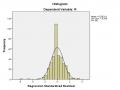
Assumptions about the normal distribution of residuals
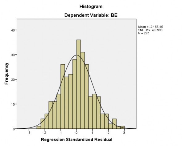
Figure 4.1. Normal distribution chart of residuals
(Source: Author's investigation results, September-October 2018)
Based on the graph, it can be said that the normal distribution of the residuals is approximately normal (Mean=- 2.1E-15) and the standard deviation Std.Dev = 0.993, which is close to 1. Therefore, it can be concluded that the assumption of normal distribution of the residuals is not violated.
We can use the PP plot chart to test this hypothesis:
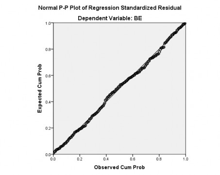
Figure 4.2. PP plot chart
(Source: Author's investigation results, September-October 2018)
Based on the PP plot, it can be seen that the observed points are not too far from the expected line, so we can conclude that the normal distribution assumption is not violated. In addition, through the scatterplot, it can be seen that there is uniform dispersion.