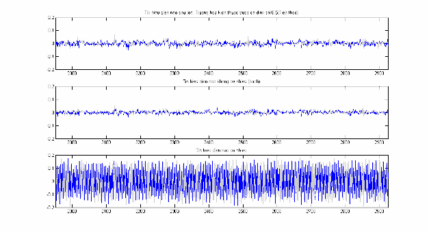
Step Size Regression Based on Absolute Value of Gradient

Figure 2.20: EEG before and after noise filtering, segment n  2001  3000 .

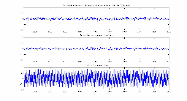
Figure 2.21: EEG before and after noise filtering, segment n  3001  4000 .

Comparison of filtered EEG signal (top) with clean EEG signal

(middle) in the next phase in figure 2.19 shows that the filtered signal reaches the noise-free EEG signal S  n  .

 ( n )

Not yet

This is also reflected in the mean square error at

Figure 2.12 and Figure 2.13. The MSE undulation increases as the step size

adaptation increases from   0.05 to   0.5 .

2.3. LMS algorithm with variable step size

The experimental results presented in the above section show a preliminary classification for the step size in using the LMS algorithm and suggest “mixing” models (see [29]), using different layers of step size to exploit the advantages of each layer. However, the proposal in [29] only solves the case of EEG signals with a strong assumption about the initial weight value. This is an important result but cannot be directly applied to the case of ECG noise filtering due to the quite different nature of these two signal layers. The distribution of the magnitude of the gradient has provided the idea and the basis for the thesis’s proposal on how to change the adaptive step size value to create a “mixing” model applicable to many different noise filtering layers in the noise filtering of ECG and EEG signals. This section introduces the mathematical basis of the method and experimental results in using a new calculation method to update the adaptive step size to filter noise during the recording of electrocardiogram and electroencephalogram signals. The experimental results illustrate and compare the performance between the proposed algorithm and the LMS algorithm with a fixed adaptive step size.

2.3.1. Step size change based on absolute value of Gradient

To speed up the convergence of the LMS algorithm, Daniel Olguín Olguín in

[29] proposed to change the adaptive step size according to the formula:

in there

  n  1    n   2 n  , (2.22)

 : Forgetting factor, has a value in the range: 0    1 , often used

choose   0.98

 : Adaptive step size parameter of  , usually chosen to satisfy

satisfy the condition   0

The above proposal originates from the problem of noise filtering for electroencephalogram (EEG) signals with the main contribution shown in formula (2.22), which is the adaptive step size change method. However, (2.22) is only suitable for the problem of noise filtering for EEG signals due to the uniform variation characteristic of this signal class with the boundary value of the signal lying in the range

 0.15   max

 0.15 (see [5], [29]). Suppression filter slot width

reflects the degree of attenuation to signals with frequencies near the current cancellation frequency

 0 (see [44]). The rejection gap width is calculated as follows:

In there:

BW : Slit width.

 2  C 2 ,

 : Adaptive step size.

C : Amplitude of the reference noise signal (see formulas 2.8 and 2.9).

Therefore, when the algorithm converges,  can take on a value small enough to make the suppression gap narrow enough. In the electrocardiogram signal (Figure 1.1), the R peak at each cycle

The activity has the characteristic of sudden change. Therefore, the calculation  2 n 

in (2.22)

may lead to failure to satisfy the stability condition of the algorithm and loss of useful information when the gap width is too large. Furthermore, the author in [29] assigns a large value of  when initializing and uses formula (2.22) to make

 decreases to the best value. This may cause the algorithm to not converge or to converge slowly if we randomly choose the initial point of the weight matrix near the minimum point.

According to [3], [27], [30], noise is also modified during the propagation from the noise source to the reference receiver. This deviation is modeled by a random quantity with Gaussian distribution. And is described in the formula

following formula:

N  n  x 1 n  normrnd  mean , sigma  . Standard deviation

sigma reflects the distance from the minimum point to the initial point of the weight matrix. The relationship between the standard deviation and the number of iterations is described in table 2.1 and in figures (2.22) and (2.23).

Table 2.1: Relationship between standard deviation and number of iterations required

for the algorithm to converge.

Standard deviation	Number of iterations required for the algorithm to converge
Standard deviation	Change step size use formula 2.20	Change step size use formula 2.21
1	0.01	500	450
2	0.005	500	400
3	0.0001	520	370
4	0.00005	520	350
5	0.000001	530	300

Maybe you are interested!

It is easy to see that if the strict assumption on the choice of initial weight values is not satisfied, the algorithm will converge slowly. Unfortunately, in many experiments, this assumption is not satisfied. The thesis proposal

based on the exploitation of information about the change in magnitude of the gradient vector in the LMS algorithm.

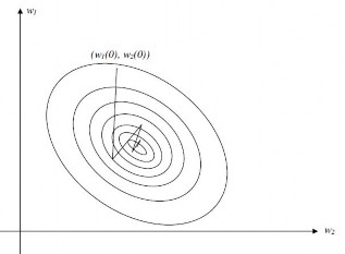
Figure 2.22: Convergence of the LMS algorithm using formula (2.22) for the control

adjust   n  , provided that the coordinates  w 1  0  , w 2  0  are chosen appropriately

Figure 2.23: Convergence of the LMS algorithm using formula (2.22) for the control

Adjust   n  , when  w 1  0  , w 2  0  are not suitable.

For a positive definite second-order function, the gradient has a large value far from the minimum point, and a small value near the minimum point (Figure 2.24). The idea

of the thesis can be described on the plane  w 1 , w 2(see [44]). At time k, the adaptive step size should take on a large value when the coordinates

1 2

 w 1  n  , w 2  n  are far from the coordinates  w * , w *  of the minimum point of the second-order performance surface (see [44]). Conversely, the adaptive step size should take the value

small when

 w 1  n  , w 2 n  is close to the coordinates of the minimum point. The choice of size

Such an adaptive step size will help the filtering algorithm satisfy the conditions on the convergence speed and stability of the algorithm. We find that the magnitude distribution of Gradient (  ) on the plane  w 1 , w 2  has properties that almost satisfy the above idea (see [38]), and the proposed adaptive step update formula is as follows:

  n  1  

x 1 n    n 



 max  x 1



 n  m m

 1,..., n  N   2

where: N is the number of samples in 1 cycle of the reference signal,

 : Ideal width for the suppression band (See [3] [29], [44])

(2.23)

 max  x 1 n m 

m  1,..., n  N  2return value C 2

at time n

 n : Step size for weight adjustment at time n .

Note that the first term of the right-hand side of (2.23)

 x 1 ( n )  ( n )

  1

  ( n )

reflects the distribution of the magnitude of the Gradient (  )

on plane  w 1 ,w 2  ,

x 1 ( n ) : Noise obtained at the reference input at time n ,

 ( n ) : Output of the noise filter at time n ,

1 2

Figure 2.24: Gradient of  on the plane ( w , w ) .

We have determined the convergence condition of the frequency cancelling filter using formula (2.23) and given in the following lemma:

Lemma . With   1

The sequences (2.11) and (2.12) with  given by (2.23) will converge.

Prove .

From formulas (2.8), (2.11) and (2.23) we have

 ( n )  S ( n )   w i ( n ) x i ( n ) , (2.24)

i  1

and

w 1 n  1   w 1 n   2  ( n  1)   n  x 1 n  ;



  2 

  1  2

 C

x ( n ) w  n  F , (2.25)

2 1   1 n

where F n

bounded by a constant M independent of n

The convergence of the above formula is reflected in the expectation of v 1 n of linear systems.

Consider the approximate linear system  v 1 ( n )  c given by



  2 

v 1 n  1    1  2

 C

x ( n )  v  n  . (2.26)

2 1   1

Expectations of

recipe

v 1 n  1 is calculated based on (2.16) and is determined by

  n   2

    

1 

2   

E  v ( n  1)     1  2

l  1  C

E  x 1 ( l )  E  v 0;





0 

  1   nE  v

(2.27)

Assume   1

ensure the convergence of the linear system. Prove the

convergence of the expectation of the sequence (2.11) with  given by (2.23) based on the evaluation (2.27) and the estimate



k  2  2  k

E   1 

l  1 

x ( l )  F

C 2 1   n  k

 M (1   ) .

Prove convergence for the sequence  w 2 n is done similarly.

2.3.2. Experiment and results

To evaluate the results, we use formula (2.7). The convergence speed of the algorithm is reflected through the convergence speed to the value of 0 or approximately 0 of MSE. The stability of the algorithm is reflected through the change of MSE after the algorithm has converged.

2.3.2.1. For electrocardiogram signals

In Figure 2.25 we show MSE in three cases.

Comment

REFERENCES

1. Nhuan Ha, Trinh Minh Hien, Tran Phuong, Hai Phong - Historical and cultural relics, Hai Phong Publishing House, 1993
2. Hai Phong City History Council, Hai Phong Gazetteer, Hai Phong Publishing House, 1990.
3. Hai Phong City History Council, History of Tien Lang District Party Committee, Hai Phong Publishing House, 1990.
4. Hai Phong City History Council, University of Social Sciences and Humanities, VNU, Hai Phong Place Names Encyclopedia, Hai Phong Publishing House. 2001.
5. Law on Cultural Heritage and documents guiding its implementation, National Political Publishing House, Hanoi, 2003.
6. Tran Duc Thanh, Lecture on Tourism Geography, Faculty of Tourism, University of Social Sciences and Humanities, VNU, 2006
7. Hai Phong Center for Social Sciences and Humanities, Some typical cultural heritages of Hai Phong, Hai Phong Publishing House, 2001
8. Nguyen Ngoc Thao (editor-in-chief, Tourism Geography, Hai Phong Publishing House, two volumes (2001-2002)
9. Nguyen Minh Tue and group of authors, Hai Phong Tourism Geography, Ho Chi Minh City Publishing House, 1997.
10. Nguyen Thanh Son, Hai Phong Tourism Territory Organization, Associate Doctoral Thesis in Geological Geography, Hanoi, 1996.
11. Decision No. 2033/QD – UB on detailed planning of Tien Lang town, Hai Phong city until 2020.
12. Department of Culture, Information, Hai Phong Museum, Hai Phong relics
- National ranked scenic spot, Hai Phong Publishing House, 2005. 13. Tien Lang District People's Committee, Economic Development Planning -
Culture - Society of Tien Lang district to 2010.
14.Website www.HaiPhong.gov.vn
APPENDIX 1
List of national ranked monuments
STT
Name of the monument
Number, year of decisiondetermine
Location
1
Gam Temple
938 VH/QĐ04/08/1992
Cam Khe Village- Toan Thang commune
2
Doc Hau Temple
9381 VH/QĐ04/08/1992
Doc Hau Village –Toan Thang commune
3
Cuu Doi Communal House
3207 VH/QĐDecember 30, 1991
Zone II of townTien Lang
4
Ha Dai Temple
Ha Dai Village –Tien Thanh commune
APPENDIX II
Number, year of decision
Phu Ke Pagoda Temple
178/QD-UBJanuary 28, 2005
Zone 1 - townTien Lang
Trung Lang Temple
Zone 4 – townTien Lang
Bao Khanh Pagoda
1900/QD-UBAugust 24, 2006
Nam Tu Village -Kien Thiet commune
Bach Da Pagoda
1792/QD-UB11/11/2002
Hung Thang Commune
5
Ngoc Dong Temple
177/QD-UBNovember 27, 2005
Tien Thanh Commune
6
Tomb of Minister TSNhu Van Lan
2848/QD-UBSeptember 19, 2003
7
Canh Son Stone Temple
2160/QD-UBSeptember 19, 2003
Van Doi Commune –Doan Lap
8
Meiji Temple
2259/QD-UBSeptember 19, 2002
Toan Thang Commune
9
Tien Doi Noi Temple
477/QD-UBSeptember 19, 2005
Doan Lap Commune
10
Tu Doi Temple
177/QD-UBJanuary 28, 2005
11
Duyen Lao Temple
Tien Minh Commune
12
Dinh Xuan Uc Pagoda
Bac Hung Commune
13
Chu Khe Pagoda
14
Dong Dinh
2848/QD-UBNovember 21, 2002
Vinh Quang Commune
15
President's Memorial HouseTon Duc Thang
NT Quy Cao
Ben Vua Temple
Tien Lang hot spring
div.maincontent .p { color: black; font-family:"Times New Roman", serif; font-style: normal; font-weight: normal; text-decoration: none; font-size: 14pt; margin:0pt; } div.maincontent p { color: black; font-family:"Times New Roman", serif; font-style: normal; font-weight: normal; text-decoration: none; font-size: 14pt; margin:0pt; } div.maincontent .s1 { color: black; font-family:"Times New Roman", serif; font-style: normal; font-weight: normal; font-size: 16pt; } div.maincontent .s2 { color: black; font-family:"Times New Roman", serif; font-style: italic; font-weight: bold; text-decoration: none; font-size: 14pt; } div.maincontent .s3 { color: black; font-family:"Times New Roman", serif; font-style: italic; font-weight: normal; text-decoration: none; font-size: 14pt; } div.maincontent .s4 { color: black; font-family:"Times New Roman", serif; font-style: normal; font-weight: normal; font-size: 14pt; } div.maincontent .s5 { color: black; font-family:"Times New Roman", serif; font-style: normal; font-weight: bold; font-size: 14pt; } div.maincontent .s6 { color: black; font-family:"Times New Roman", serif; font-style: normal; font-weight: normal; text-decoration: none; font-size: 14pt; } div.maincontent .s7 { color: black; font-family:"Times New Roman", serif; font-style: normal; font-weight: bold; text-decoration: none; font-size: 14pt; } div.maincontent .s8 { color: black; font-family:"Times New Roman", serif; font-style: normal; font-weight: normal; text-decoration: none; font-size: 9pt; vertical-align: 6pt; } div.maincontent .s9 { color: black; font-family:"Times New Roman", serif; font-style: normal; font-weight: bold; text-decoration: none; font-size: 12pt; } div.maincontent .s11 { color: black; font-family:"Times New Roman", serif; font-style: normal; font-weight: normal; tex
Solutions for tourism development in Tien Lang - 10
zt2i3t4l5ee
zt2a3gstourism, tourism development
zt2a3ge
zc2o3n4t5e6n7ts
- District People's Committees and authorities of communes with tourist attractions should support, promote, and provide necessary information to people, helping them improve their knowledge about tourism. Raise tourism awareness for local people.
*
* *
Due to limited knowledge and research time, the thesis inevitably has shortcomings. Therefore, I look forward to receiving guidance from teachers, experts as well as your comments to make the thesis more complete.
Chapter III Conclusion
Through the issues presented in Chapter II, we can come to some conclusions:
Based on the strengths of available tourism resources, the types of tourism in Tien Lang that need to be promoted in the coming time are sightseeing and resort tourism, discovery tourism, weekend tourism. To improve the quality and diversify tourism products, Tien Lang district needs to combine with local cultural tourism resources, at the same time combine with surrounding areas, build rich tourism products. The strengths of Tien Lang tourism are eco-tourism and cultural tourism, so developing Tien Lang tourism must always go hand in hand with restoring and preserving types of cultural tourism resources. Some necessary measures to support and improve the efficiency of exploiting tourism resources in Tien Lang are: strengthening the construction of technical facilities and labor force serving tourism, actively promoting and advertising tourism, and expanding forms of capital mobilization for tourism development.
CONCLUDE
I Conclusion
1. Based on the results achieved within the framework of the thesis's needs, some basic conclusions can be drawn as follows:
Tien Lang is a locality with great potential for tourism development. The relatively abundant cultural tourism resources and ecological tourism resources have great appeal to tourists. Based on this potential, Tien Lang can build a unique tourism industry that is competitive enough with other localities within Hai Phong city and neighboring areas.
In recent years, the exploitation of the advantages of resources to develop tourism and build tourist routes in Tien Lang has not been commensurate with the available potential. In terms of quantity, many resource objects have not been brought into the purpose of tourism development. In terms of time, the regular service time has not been extended to attract more visitors. Infrastructure and technical facilities are still weak. The labor force is still thin and weak in terms of expertise. Tourism programs and routes have not been organized properly, the exploitation content is still monotonous, so it has not attracted many visitors. Although resources have not been mobilized much for tourism development, they are facing the risk of destruction and degradation.
2. Based on the results of investigation, analysis, synthesis, evaluation and selective absorption of research results of related topics, the thesis has proposed a number of necessary solutions to improve the efficiency of exploiting tourism resources in Tien Lang such as: promoting the restoration and conservation of tourism resources, focusing on investment and key exploitation of ecotourism resources, strengthening the construction of infrastructure and tourism workforce. Expanding forms of capital mobilization. In addition, the thesis has built a number of tourist routes of Hai Phong in which Tien Lang tourism resources play an important role.
Exploiting Tien Lang tourism resources for tourism development is currently facing many difficulties. The above measures, if applied synchronously, will likely bring new prospects for the local tourism industry, contributing to making Tien Lang tourism an important economic sector in the district's economic structure.
div.maincontent .p { color: black; font-family:"Times New Roman", serif; font-style: normal; font-weight: normal; text-decoration: none; font-size: 14pt; margin:0pt; } div.maincontent p { color: black; font-family:"Times New Roman", serif; font-style: normal; font-weight: normal; text-decoration: none; font-size: 14pt; margin:0pt; } div.maincontent .s1 { color: black; font-family:"Times New Roman", serif; font-style: normal; font-weight: normal; font-size: 16pt; } div.maincontent .s2 { color: black; font-family:"Times New Roman", serif; font-style: italic; font-weight: bold; text-decoration: none; font-size: 14pt; } div.maincontent .s3 { color: black; font-family:"Times New Roman", serif; font-style: italic; font-weight: normal; text-decoration: none; font-size: 14pt; } div.maincontent .s4 { color: black; font-family:"Times New Roman", serif; font-style: normal; font-weight: normal; font-size: 14pt; } div.maincontent .s5 { color: black; font-family:"Times New Roman", serif; font-style: normal; font-weight: bold; font-size: 14pt; } div.maincontent .s6 { color: black; font-family:"Times New Roman", serif; font-style: normal; font-weight: normal; text-decoration: none; font-size: 14pt; } div.maincontent .s7 { color: black; font-family:"Times New Roman", serif; font-style: normal; font-weight: bold; text-decoration: none; font-size: 14pt; } div.maincontent .s8 { color: black; font-family:"Times New Roman", serif; font-style: normal; font-weight: normal; text-decoration: none; font-size: 9pt; vertical-align: 6pt; } div.maincontent .s9 { color: black; font-family:"Times New Roman", serif; font-style: normal; font-weight: bold; text-decoration: none; font-size: 12pt; } div.maincontent .s11 { color: black; font-family:"Times New Roman", serif; font-style: normal; font-weight: normal; tex -
Car body electrical practice - 8
zt2a3gs
If the voltage is out of specification, replace the wire or connector.
If the voltage is within specification, install the front fog light relay and follow step 5.
Step 5 Check the front fog light switch
- Remove the D4 connector of the fog light switch
- Use a multimeter to measure the resistance of the front fog light switch.
Measurement location
Condition
Standard
D4-3 (BFG) -D4-4 (LFG)
Light switchFront Fog OFF
>10kΩ
Front fog light switchON
<1 Ω
- Standard resistor
D4 connector is located on the combination switch assembly.
If the resistance is out of specification, replace the combination switch (the fog light switch is located in the combination switch).
If the resistance is within specification, follow step 6.
Step 6 Check wiring and connectors (front fog light relay-light selector switch)
- Disconnect connector D4 of the combination switch assembly
- Use a voltmeter to measure the voltage value of jack D4 on the wire side.
Control modecontrol
D4-3 (BFG) - (-) AQ
TAIL
11 to 14 V
D4 connector for the wiring of the combination switch assembly
If the voltage does not meet the standard, replace the wire or connector.
If the voltage is within standard, there may have been an error in the previous measurements.
Step 7 Check the front fog lights
- Remove the front fog light electrical connector.
- Supply battery voltage to the fog lamp terminals
Jack 8, B9 of front fog lamp on the electrical side
blind first.
Power supply location
Terms and Conditions
Battery positive terminal - Terminal 2Battery negative terminal - Terminal 1
Fog lightsbefore morning
- If the light does not come on, replace the bulb.
If the light is on, re-plug the jack and continue to step 8.
Step 8 Check wiring and connectors (relay and front fog lights)
- Disconnect the B8 and B9 connectors of the front fog lights.
- Use a voltmeter to measure voltage at the following locations:
Switch location
B8-2 - (-) AQ
Electric lock ON TAIL size switchFog switch ON
B9-2 - (-) AQ
Electric lock ONTAIL size switch Fog switch ON
B8 and B9 connectors on the front fog lamp wiring side
Voltage is not up to standard, repair or replace the jack. If up to standard, there may have been an error in the measurement process.
2.2.4. Procedure for removing, installing and adjusting fog lights 1. Procedure for removing
- Remove the front inner ear pads
Use a screwdriver to remove the 3 screws and remove the front part of the front inner ear liner
-Remove the fog light assembly
+ Disconnect the connector.
+ Use a screwdriver to remove 3 screws to remove the fog light cover
2. Installation sequence
-Rotate the fog lamp bulb in the direction indicated by the arrow as shown in the figure and remove the fog lamp from the fog lamp assembly.
-Rotate the fog light bulb in the direction indicated by the arrow as shown in the figure and install the light into the fog light assembly.
- Use a screwdriver to install the fog light cover
-Install the electrical connector
Attention: Be careful not to damage the plastic thread on the lamp assembly.
- Install the front inner ear pads
Use a screwdriver to install the front inner bumper with 3 screws.
3. Prepare the vehicle to adjust the fog light convergence. Prepare the vehicle:
- Make sure there is no damage or deformation to the vehicle body around the fog lights.
- Add fuel to the fuel tank
- Add oil to standard level.
- Add engine coolant to standard level.
- Inflate the tire to standard pressure.
- Place spare tire, tools and jack in original design position
- Do not leave any load in the luggage compartment.
- Let a person weighing about 75 kg sit in the driver's seat.
4. Prepare to check the fog light convergence
a/ Prepare the vehicle status as follows:
- Place the car in a dark enough place to see the lines. The lines are the dividing line, below which the light from the fog lights can be seen but above which it cannot.
- Place the car perpendicular to the wall.
- Keep a distance of 7.62 m between the center of the fog lamp and the wall.
- Park the car on level ground.
- Press the car down a few times to stabilize the suspension.
Note: A distance of approximately 7.62 m is required between the vehicle (fog lamp center) and the wall to adjust the convergence correctly. If the distance of 7.62 m cannot be achieved, set the correct distance of 3 m to check and adjust the fog lamp convergence. (Since the target area varies with the distance, please follow the instructions as shown in the figure.)
b/ Prepare a piece of thick white paper about 2 m high and 4 m wide to use as a screen.
c/ Draw a vertical line through the center of the screen (line V).
d/ Set the screen as shown in the picture. Note:
- Keep the screen perpendicular to the ground.
- Align the V line on the screen with the center of the vehicle.
e/Draw the reference lines (H, V LH and V RH lines) on the screen as shown in the figure.HINT:
Mark the center of the fog lamp on the screen. If the center mark cannot be seen on the fog lamp, use the center of the fog lamp or the manufacturer's name mark on the fog lamp as the center mark.
H line (fog light height):
Draw a line across the screen so that it passes through the center mark. Line H should be at the same height as the center mark of the fog light bulb.
Line V LH, V RH (center mark position of left fog lamp LH and right fog lamp RH):
Draw two lines so that they intersect line H at the center marks.
5. Check the fog light convergence
a/ Cover the fog lamp or remove the connector of the other side fog lamp to prevent light from the unchecked fog lamp from affecting the fog lamp convergence test.
b/ Start the engine.
c/ Turn on the fog lights and make sure that the dividing line is outside the standard area as shown in the drawing.
6. Adjust the fog light convergence
Use a screwdriver to adjust the fog light to the standard area by turning the toe adjustment screw.
Note: If the screw is adjusted too far, loosen it and then tighten it again, so that the last rotation of the light adjustment screw is clockwise.
3. Self-study questions
1. Describe the operating principle of the lighting system with automatic headlight function
2. Describe the operating principle of the lighting system with the function of rotating headlights when turning
3. Draw diagram and connect lighting system on Hyundai Porter car
4. Draw diagram and connect lighting system on Honda Accord 1992
5. Draw the lighting circuit on a 1993 Toyota Lexus
LESSON 3 MAINTENANCE AND REPAIR OF SIGNAL SYSTEM
I. IMPLEMENTATION GOAL
After completing this lesson, students will be able to:
- Distinguish between types of signals on cars
- Correctly describe common symptoms and suspected areas causing damage.
- Connecting signal circuits ensures technical requirements
- Disassemble, install, check, maintain and repair the signal system to ensure technical requirements.
- Ensure safety in work and industrial hygiene
II. LESSON CONTENT
1. General description
The signal system equipped on cars aims to create signals to notify other vehicles participating in traffic about the vehicle's operating status such as: stopping, parking, braking, reversing, turning...
Signals are used either by light such as headlamps, brake lights, turn signals….. or by sound such as horns, reverse music….
Just like the lighting system. A signal system circuit usually consists of: battery, fuse, wire, relay, electrical load and control switch. Only some switches of the signal system are on the combination switch. The switches of other signals are usually located in different locations such as in the gearbox or brake pedal……
2. Maintenance and repair
2.1. Turn signals and hazard lights
The installation location of the turn signal is shown in Figure 3.1. The turn signal control switch is located in the combination switch under the steering wheel. Turning this switch to the right or left will make the turn signal turn right or left.
The hazard light switch is used when the vehicle has a problem while participating in traffic. When the hazard light switch is turned on, all the turn signals on the vehicle will light up at a certain frequency. The hazard light switch is usually placed separately from the turn signal switch (some old cars integrate the hazard and turn signal switches on the same combination switch cluster).
Figure 3.1 Turn signal switch Figure 3.2 Hazard switch
The part that generates the flashing frequency for the lights is called a turn signal relay. The turn signal relay usually has 3 terminals: B (positive power supply); E (negative power supply); L (providing the turn signal switch to distribute to the
lamp)
2.1.1. Circuit diagram
To generate the frequency for the turn signal, a turn signal relay is used in the turn signal circuit. The current from the turn signal relay will be sent to the turn signal switch assembly to distribute the current to the turn signal lights for the driver's purpose.
Figure 3.3. Schematic diagram of a turn signal circuit without a hazard switch
1. Battery; 2. Electric lock; 3. Turn signal relay; 4. Turn signal switch; 5. Turn signal lamp; 6. Turn signal lamp; 7. Hazard switch
Figure 3.4 Schematic diagram of turn signal circuit with hazard switch
1. Battery; 2. Combination switch cluster; 3. Turn signal;
4. Turn signal light; 5. Turn signal relay
Today's cars no longer use three-pin turn signal relays (B, L, E) but use eight-pin turn signal relays (figure 3.5) (pin number 8 is used for hazard lights).
For this type, the current supplying the turn signal lights is supplied directly from the turn signal relay to the lights.
div.maincontent .p { color: black; font-family:"Times New Roman", serif; font-style: normal; font-weight: normal; text-decoration: none; font-size: 14pt; margin:0pt; } div.maincontent p { color: black; font-family:"Times New Roman", serif; font-style: normal; font-weight: normal; text-decoration: none; font-size: 14pt; margin:0pt; } div.maincontent .s1 { color: black; font-family:"Times New Roman", serif; font-style: normal; font-weight: normal; text-decoration: none; font-size: 13pt; } div.maincontent .s2 { color: black; font-family:"Times New Roman", serif; font-style: italic; font-weight: normal; text-decoration: none; font-size: 14pt; } div.maincontent .s3 { color: black; font-family:"Times New Roman", serif; font-style: normal; font-weight: normal; text-decoration: none; font-size: 14pt; } div.maincontent .s4 { color: black; font-family:"Times New Roman", serif; font-style: normal; font-weight: normal; text-decoration: none; font-size: 13pt; } div.maincontent .s5 { color: black; font-family:"Times New Roman", serif; font-style: normal; font-weight: normal; text-decoration: none; font-size: 13pt; vertical-align: 1pt; } div.maincontent .s6 { color: black; font-family:"Times New Roman", serif; font-style: normal; font-weight: normal; text-decoration: none; font-size: 11pt; } div.maincontent .s7 { color: black; font-family:"Times New Roman", serif; font-style: normal; font-weight: normal; text-decoration: none; font-size: 14pt; vertical-align: -9pt; } div.maincontent .s8 { color: black; font-family:"Times New Roman", serif; font-style: normal; font-weight: normal; text-decoration: none; font-size: 11pt; } div.maincontent .s9 { color: #008000; font-family:"Times New Roman", serif; font-style: normal; font-weight: normal; text-decoration: none; font-size: 14pt; } div.maincontent .s10 { color: black; font-family:"Times New Roman", serif; font-style: italic; font-weight: normal; te
div.maincontent .p { color: black; font-family:"Times New Roman", serif; font-style: normal; font-weight: normal; text-decoration: none; font-size: 14pt; margin:0pt; } div.maincontent p { color: black; font-family:"Times New Roman", serif; font-style: normal; font-weight: normal; text-decoration: none; font-size: 14pt; margin:0pt; } div.maincontent .s1 { color: black; font-family:"Times New Roman", serif; font-style: normal; font-weight: normal; text-decoration: none; font-size: 13pt; } div.maincontent .s2 { color: black; font-family:"Times New Roman", serif; font-style: italic; font-weight: normal; text-decoration: none; font-size: 14pt; } div.maincontent .s3 { color: black; font-family:"Times New Roman", serif; font-style: normal; font-weight: normal; text-decoration: none; font-size: 14pt; } div.maincontent .s4 { color: black; font-family:"Times New Roman", serif; font-style: normal; font-weight: normal; text-decoration: none; font-size: 13pt; } div.maincontent .s5 { color: black; font-family:"Times New Roman", serif; font-style: normal; font-weight: normal; text-decoration: none; font-size: 13pt; vertical-align: 1pt; } div.maincontent .s6 { color: black; font-family:"Times New Roman", serif; font-style: normal; font-weight: normal; text-decoration: none; font-size: 11pt; } div.maincontent .s7 { color: black; font-family:"Times New Roman", serif; font-style: normal; font-weight: normal; text-decoration: none; font-size: 14pt; vertical-align: -9pt; } div.maincontent .s8 { color: black; font-family:"Times New Roman", serif; font-style: normal; font-weight: normal; text-decoration: none; font-size: 11pt; } div.maincontent .s9 { color: #008000; font-family:"Times New Roman", serif; font-style: normal; font-weight: normal; text-decoration: none; font-size: 14pt; } div.maincontent .s10 { color: black; font-family:"Times New Roman", serif; font-style: italic; font-weight: normal; te -
![Qos Assurance Methods for Multimedia Communications
low. The EF PHB requires a sufficiently large number of output ports to provide low delay, low loss, and low jitter.
EF PHBs can be implemented if the output ports bandwidth is sufficiently large, combined with small buffer sizes and other network resources dedicated to EF packets, to allow the routers service rate for EF packets on an output port to exceed the arrival rate λ of packets at that port.
This means that packets with PHB EF are considered with a pre-allocated amount of output bandwidth and a priority that ensures minimum loss, minimum delay and minimum jitter before being put into operation.
PHB EF is suitable for channel simulation, leased line simulation, and real-time services such as voice, video without compromising on high loss, delay and jitter values.
Figure 2.10 Example of EF installation
Figure 2.10 shows an example of an EF PHB implementation. This is a simple priority queue scheduling technique. At the edges of the DS domain, EF packet traffic is prioritized according to the values agreed upon by the SLA. The EF queue in the figure needs to output packets at a rate higher than the packet arrival rate λ. To provide an EF PHB over an end-to-end DS domain, bandwidth at the output ports of the core routers needs to be allocated in advance to ensure the requirement μ > λ. This can be done by a pre-configured provisioning process. In the figure, EF packets are placed in the priority queue (the upper queue). With such a length, the queue can operate with μ > λ.
Since EF was primarily used for real-time services such as voice and video, and since real-time services use UDP instead of TCP, RED is generally
not suitable for EF queues because applications using UDP will not respond to random packet drop and RED will strip unnecessary packets.
2.2.4.2 Assured Forwarding (AF) PHB
PHB AF is defined by RFC 2597. The purpose of PHB AF is to deliver packets reliably and therefore delay and jitter are considered less important than packet loss. PHB AF is suitable for non-real-time services such as applications using TCP. PHB AF first defines four classes: AF1, AF2, AF3, AF4. For each of these AF classes, packets are then classified into three subclasses with three distinct priority levels.