also gives us a dot product.
There are many ways to construct the dot product by definition, as long as we have a positive definite symmetric bilinear form (according to Sylvester's criterion, all the main sub-determinants of the matrix representation are positive) we get a dot product.
The real vector space V on which a dot product is equipped is called
Euclidean space .
Below we give some important scalar product inequalities.
Maybe you are interested!
-
 Summary of Sem Linear Structural Model Data
 -
 Training creative thinking for high school students through solving some Algebra - Analysis exercises in many ways - 6
 -
 Results of Linear Regression Analysis on Factors Affecting Land Complaints in Vinh City
 -
 Simple Iteration Method to Solve Linear Equations
 -
 Detecting Essential Assumption Violations in Linear Regression
3.2.2 Scalar product inequality

Cauchy - Bunhia - Schwartz (CBS) inequality
Theorem 3.2.1. (Cauchy - Bunhia - Schwartz inequality)
⟨ x, y ⟩ 2 6 ⟨ x, x ⟩ ⟨ y, y ⟩ (3.7)
Proof: If x = 0 or y = 0 the inequality is obviously true.
Suppose x, y ̸ = 0 , we have
⟨ x + λy, x + λy ⟩ > 0 , ∀ x, y ∈ V, λ ∈ R
expand we get
λ 2 ⟨ y, y ⟩ + 2 λ ⟨ x, y ⟩ + ⟨ x, x ⟩ > 0 , ∀ x, y ∈ V, λ ∈ R
This is a quadratic trinomial that holds for all λ ∈ R if and only if
⟨ x, y ⟩ 2− ⟨ x, x ⟩ ⟨ y, y ⟩ 6 0
Equality occurs if x + λy = 0 , that is, x, y are linearly dependent. I
√
Minkowski inequality
For every x ∈ V then ⟨ x, y ⟩ ≥ 0 , we define the number ∥ x ∥ = ⟨ x, x ⟩ and call it the norm of vector x (sometimes also called the modulus or length of x ). It is not difficult to see that ∥ x ∥ has the following properties:
i) ∥ x ∥ ≥ 0 , ∀ x ∈ V, the equality occurs if and only if x = 0 .
ii) ∥ λx ∥ = | λ | ∥ x ∥ , ∀ x ∈ V, λ ∈ R .
iii) ∥ x + y ∥ 6 ∥ x ∥ + ∥ y ∥ , equality occurs if and only if x, y are linearly dependent.
The last property is the Minkowski inequality. We prove this inequality. We have
2 2 2
∥ x + y ∥ = ⟨ x, x ⟩ + 2 ⟨ x, y ⟩ + ⟨ y, y ⟩ = ∥ x ∥ + 2 ⟨ x, y ⟩ + ∥ y ∥
Using the CBS inequality we have
2 2 2 2
∥ x + y ∥ 6 ∥ x ∥ + 2 ∥ x ∥ ∥ y ∥ + ∥ y ∥ = ( ∥ x ∥ + ∥ y ∥ )
And it is easy to obtain the Minkowski inequality. The equality holds if and only if x, y are linearly dependent.
A space V is called normed if for every x ∈ V it determines a
The standard satisfies conditions i)-iii) above.
The norm ∥ x − y ∥ is called the distance between x and y , denoted d ( x, y ) .
This distance is of a nature.
d ( x, y ) ≤ d ( x, z ) + d ( z, y )
and is called the triangle inequality, which follows directly from the Minkowski inequality.
3.2.3 Orthonormal basis, Gram-Schmidt orthonormalization process
Suppose on V equipped with a dot product. Two vectors are called orthogonal , denoted x ⊥ y if ⟨ x, y ⟩ = 0 .
∑
Proposition 3.2.1. Suppose v 1 , .., v m ∈ V are orthogonal pairwise vectors, then
2
m
i =1
2
for
m
∑
=
i =1
∥ v i ∥
The above proposition is easily proven. When m = 2 we have the Pythagorean formula .
The vector system { e 1 , ..., e m } in V is called orthogonal if e i ̸ = 0 and e i ⊥ e j
for all i ̸ = j, where i, j = 1; m , that is,
⟨ e i , e j
⟩ = {0 , i ̸ = j
2
∥ e i ∥ , i = j
An orthogonal system for which ∥ e i ∥ = 1 is called an orthonormal system .
Proposition 3.2.2. Orthogonal systems are linearly independent.
A basis { e 1 , ..., e n } is called an orthonormal basis if it is an orthonormal system.
|| e i ||
If { e 1 , ..., e n } is an orthogonal basis then { e ′ 1 , ..., e ′ n } , where e ′ i =e i, is an orthonormal basis. Such a process is called orthonormal basis normalization .
Theorem 3.2.2. (Gram-Schmidt) If the system of vectors { v 1 , ..., v m } is linearly independent in V, then there exists an orthonormal system { e 1 , ..., e m } such that e i ∈ Span { v 1 , ..., v i } , ∀ i = 1; m .
Proof: We prove by induction.
|| v 1 ||
With j = 1 , let e 1 =v 1. Suppose we can construct the orthonormal system { e 1 , ..., e j } and e k ∈ span { v 1 , ..., v k } , ∀ k = 1; j . We show how to construct e j +1 .
Let e ′ j +1 = v j +1 + α 1 e 1 + ... + α j e j , where the α i are defined as follows and require
e ′ j +1 ⊥ e k , ∀ k = 1; j . Thus
⟨ e ′ j +1 , e k ⟩ = 0 ⇔ ⟨ v j +1 , e k ⟩ + α k ∥ e k ∥ = 0
Since ∥ e k ∥ = 1 , α k = − ⟨ v j +1 , e k ⟩ , ∀ k = 1; j That is,
∑
j
e ′ j +1 = v j +1 − ⟨ v j +1 , e k ⟩ e k
k =1
Since { v 1 , ..., v j , v j +1 } are linearly independent, v j +1 is not linearly representable by { e 1 , ..., e j } (since span { e 1 , ..., e j } = span { v 1 , ..., v j } ), so e ′ j +1 ̸ = 0 .
Put
e j +1 =
e ′ j +1
e ′ j +1
We get the orthonormal system { e 1 , ..., e j +1 } satisfying the theorem. I
Corollary 3.2.1. If { v 1 , ..., v n } is any basis of V then there exists an orthonormal basis { e 1 , ..., e n } such that e j ∈ span { v 1 , ..., v j } .
Theorem 3.2.3. If { e 1 , ..., e n } is an orthonormal basis of V then for every
x ∈ V we have
∑
n
x = ⟨ x, e i ⟩ e i .
i =1
The theorem can be proved easily.
Note 11. Thus every n- dimensional Euclidean vector space V has an orthonormal basis. Any orthonormal system in space V can be supplemented so that
∑
∑
form an orthonormal basis. Suppose { e 1 , ..., e n } is an orthonormal basis, then with
for all x, y ∈ V where x =
n
i =1
n
x i e i , y = y i e i we have
i =1
n
⟨ x, y ⟩ = ∑x i y i
i =1
∥ x ∥ = t
x 2
i
v u ∑ n.
i =1
i =1
Proposition 3.2.3. Suppose there are two orthonormal bases { e 1 , ..., e n } and { e ′ 1 , ..., e ′ n } in the Euclidean space V . Then the basis transformation matrix C : ( e ) → ( e ′ ) is an orthogonal matrix.
Proof: We have ( e ′ ) = ( e ) C , therefore ( e ′ ) T = C T ( e ) T . Consider the matrix of scalar products
( e ′ ) T ( e ′ ) =
. . .
. . . . .
⟨ e ′ 1 , e ′ 1 ⟩ · · . · ⟨ e ′ 1 , e ′ n ⟩
= E
n
1
.
n
n
⟨ e ′ , e ′ ⟩ . . ⟨ e ′ , e ′ ⟩
similarly then ( e ) T ( e ) = E , which means that
C T ( e ) T ( e ) C = C T EC = C T C = E
or C T = C − 1 . I
Example 85. Gram-schmidt orthonormalization of vector systems
v 1 = (1 , 1 , 1) , v 2 = (0 , 1 , 1) , v 3 = (0 , 0 , 1)
It is clear that this system is linearly independent.
Let w 1 = v 1 , e 1 =w 1
|| w 1 ||
=( √ 1
, 1 ,1
√
√
⇒ e 2 =
=
3 3
) . Next, we have
3
w 2= v 2− ⟨ v 2 , e 1 ⟩ e 1=
−
,
,
( 211 )
w 2 (
−√, √, √
2 1 1 )
3 3 3
and
∥ w 2 ∥
6 6 6
w = v − ⟨ v , e ⟩ e
− ⟨ v , e ⟩ e = ( 0 , − 1 , 1 )
since
3 3 3 1 1
3 2 2 2 2
e 3 =
=
∥
0 , −√ 2 , √ 2
w 3 (
3
1 1 )
∥ w
3
The matrix that transforms an orthonormal basis to an orthonormal one is an orthogonal matrix, so orthogonal matrices play an important role. The following example shows all the forms of second-order orthogonal matrices.
Example 86. Find the representation of a second-order orthogonal matrix. Suppose the matrix
(
)
Second order orthogonality has the form
A = abcd
According to the hypothesis AA T= E , so det( A ) = ± 1 . From there we have the system of equations to find the elements of A as
a 2 + c 2 = 1
ab + c d = 0
b 2 + d 2 = 1
a d − bc = 1
or
a 2 + c 2 = 1
ab + c d = 0
b 2 + d 2 = 1
(
a d − bc = − 1
Solving the system, we find matrix A has only two representations:
or
A = ab
- three
(
A = ab
b − a
) , a 2 + b 2 = 1
) , a 2 + b 2 = 1
Let a = cos φ, b = sin φ then we rewrite A in the form
or
A = cos φ sin φ
(
)
− sin φ cos φ
(
)
A = cos φ sin φ
sin φ − cos φ
3.2.4 QR Analysis
Suppose that A ∈ M n × m ( R ) is a matrix of m linearly independent columns, A is written in the form of column vectors as A = ( v 1 , v 2 , ..., v m ) . Gram-Schmidt orthonormalization of vectors v 1 , v 2 , ..., v mwe get the vectors e 1 , e 2 , ..., e m , on the other hand from the proof of theorem 3.2.2 we see that
∑
k
v k = ⟨ v k , e i ⟩ e i
i =1
so we can write
⟨ v 1 , e 1 ⟩ ⟨ v 2 , e 1 ⟩ · · · ⟨ v m , e 1 ⟩
.
.
.
.
A = ( v , v
, ..., and
) = ( e , e
, ..., e
)
0 ⟨ v 2 , e 2 ⟩ · · · ⟨ v m , e 2 ⟩
.
.
.
.
= QR
1 2 m
1 2 m .
. . .
.
. . .
0 0 · · · ⟨ v m , e m ⟩
Thus Q is a matrix of orthogonal columns, and R is a square matrix of order m of coefficients when expanding the vectors v k in the orthonormal basis obtained from the Gram-Schmidt orthonormalization of these vectors (Fourier coefficients). Clearly ⟨ v i , e i ⟩ ̸ = 0 so R is invertible. We can state this result in the form of the following theorem.
Theorem 3.2.4. Suppose A ∈ M n × m ( R ) with rank ( A ) = m , then we can analyze
A = QR
where Q is a matrix with orthogonal columns, and R is an invertible upper triangular matrix of order m .
From the above theorem we see that if A is an invertible square matrix of order n , then Q is an orthogonal matrix of order n . One more thing to note is that QR decomposition is not unique in general.
Example 87. Given matrix
1 0 0
A = ( v 1 , v 2 , v 3 ) = 1 1 0
1 1 1
Find a QR decomposition of it. To solve the problem, we first directly
Gram-Schmidt normalization of vectors v 1 , v 2 , v 3 , for example we find
e 1 =
√ 3 , √ 3 , √ 3
, e 2 =
−√ 6 , √ 6 , √ 6
, e 3 =
0 , −√ 2 , √ 2
(1 1 1 ) T (2 1 1 ) T (1 1 ) T
At that time
Still
1
√
√
√
3
3
1
3
Q = 1
− √ 6
2
√
1
6
√
1
6
0
1
− √ 2
√
1
2
⟨ v 1 , e 1 ⟩ ⟨ v 2 , e 1 ⟩ ⟨ v 3 , e 1 ⟩
√ 3 2 1
√
√
√
√
6 6
3 3
R =
0 ⟨ v 2 , e 2 ⟩ ⟨ v 3 , e 2 ⟩ = 0
2 1
√
0 0 ⟨ v 3 , e 3 ⟩
0 0 1
2
3.3 Orthogonal subspaces and projections
Definition 44. Suppose V is a real Euclidean space, W, Z are two subspaces of V . W and Z are called orthogonal, written as W ⊥ Z , if w ⊥ z, ∀ w ∈ W, z ∈ Z. If V = W ⊕ Z and W ⊥ Z then W, Z are orthogonal complementary subspaces.
Proposition 3.3.1. Suppose W, Z are subspaces of Eulcid space
V.
a) { 0 } ⊥ W for all W - subspaces of V .
b) If W ⊥ Z then W ∩ Z = { 0 } .
c) W ⊥ = { v ∈ V : v ⊥ w, ∀ w ∈ W } is the orthogonal complement of W .
Suppose x, y are non -zero vectors in Euclidean space V , the angle between x
d
and y denotes x, y ∈ [0 , π ] determined from
c os ( x, y ) = ⟨ x, y ⟩
d ∥ x ∥ ∥ y ∥
Theorem 3.3.1. Suppose V is an n- dimensional Euclidean space , { v 1 , ..., v m } is an orthonormal system of vectors in V , W = span { v 1 , ..., v m } , for all x ∈ V , let
∑
m
w 1 = ⟨ x, v i ⟩ v i
i =1
w 2 = x − w 1
At that time
a) w 1 ∈ W
b) w 2 ⊥ W .
Prove:
a) Obviously.
b) We have
2
⟨ w 2 , v i ⟩ = ⟨ x − w 1 , v i ⟩ = ⟨ x, v i ⟩ − ⟨ x, v i ⟩ ∥ v i ∥ = 0
Therefore w 2 ⊥ W . I
Vector w 1 is called the projection of x onto W , denoted w 1 = ch W x , and w 2 is called the component of x orthogonal to W .
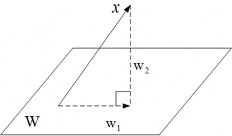
Figure 3.2: Orthogonal projection
Proposition 3.3.2. Suppose vector v ∈ V and W is a subspace of V , then
w ∈ W
min ∥ v − w ∥ = ∥ v − ch W v ∥
Proof: Let v 0 = ch W v , we have
2
∥ v − w ∥ = ⟨ v − w, v − w ⟩ = ⟨ v − v 0 + v 0 − w, v − v 0 + v 0 − w ⟩
2 2 2 2
= ∥ v − v 0 ∥ + ∥ v 0 − w ∥ + 2 ⟨ v − v 0 , v 0 − w ⟩ = ∥ v − v 0 ∥ + ∥ v 0 − w ∥
since v 0 − w ∈ W, v − v 0 ∈ W ⊥ . Therefore
∥ v − w ∥ > ∥ v − v 0 ∥
The equality sign holds if and only if w = v 0 . I
3.4 Diagonalization of symmetric matrices
3.4.1 Self-adjoint operators
Definition 45. Suppose V is a real Euclidean space, a linear operator f : V → V is called self-adjoint (or symmetric) if for all x, y ∈ V we have
⟨ f ( x ) , y ⟩ = ⟨ x, f ( y ) ⟩