RBF NEURAL NETWORK
1.3.1 Radial basis function technique and RBF neural network
Radial basis function was introduced by MJD Powell to solve multivariate function interpolation problem in 1987. In the field of neural network, RBF neural network was proposed by DS Bromhead and D. Lowe in 1988 for multivariate function interpolation and approximation problem (see [5]).
Below we will briefly present the technique of using radial basis functions to solve multivariate interpolation problems.
Radial basis function technique
Maybe you are interested!
-
![Qos Assurance Methods for Multimedia Communications
zt2i3t4l5ee
zt2a3gs
zt2a3ge
zc2o3n4t5e6n7ts
low. The EF PHB requires a sufficiently large number of output ports to provide low delay, low loss, and low jitter.
EF PHBs can be implemented if the output ports bandwidth is sufficiently large, combined with small buffer sizes and other network resources dedicated to EF packets, to allow the routers service rate for EF packets on an output port to exceed the arrival rate λ of packets at that port.
This means that packets with PHB EF are considered with a pre-allocated amount of output bandwidth and a priority that ensures minimum loss, minimum delay and minimum jitter before being put into operation.
PHB EF is suitable for channel simulation, leased line simulation, and real-time services such as voice, video without compromising on high loss, delay and jitter values.
Figure 2.10 Example of EF installation
Figure 2.10 shows an example of an EF PHB implementation. This is a simple priority queue scheduling technique. At the edges of the DS domain, EF packet traffic is prioritized according to the values agreed upon by the SLA. The EF queue in the figure needs to output packets at a rate higher than the packet arrival rate λ. To provide an EF PHB over an end-to-end DS domain, bandwidth at the output ports of the core routers needs to be allocated in advance to ensure the requirement μ > λ. This can be done by a pre-configured provisioning process. In the figure, EF packets are placed in the priority queue (the upper queue). With such a length, the queue can operate with μ > λ.
Since EF was primarily used for real-time services such as voice and video, and since real-time services use UDP instead of TCP, RED is generally
not suitable for EF queues because applications using UDP will not respond to random packet drop and RED will strip unnecessary packets.
2.2.4.2 Assured Forwarding (AF) PHB
PHB AF is defined by RFC 2597. The purpose of PHB AF is to deliver packets reliably and therefore delay and jitter are considered less important than packet loss. PHB AF is suitable for non-real-time services such as applications using TCP. PHB AF first defines four classes: AF1, AF2, AF3, AF4. For each of these AF classes, packets are then classified into three subclasses with three distinct priority levels.
Table 2.8 shows the four AF classes and 12 AF subclasses and the DSCP values for the 12 AF subclasses defined by RFC 2597. RFC 2597 also allows for more than three separate priority levels to be added for internal use. However, these separate priority levels will only have internal significance.
PHB Class
PHB Subclass
Package type
DSCP
AF4
AF41
Short
100010
AF42
Medium
100100
AF43
High
100110
AF3
AF31
Short
011010
AF32
Medium
011100
AF33
High
011110
AF2
AF21
Short
010010
AF22
Medium
010100
AF23
High
010110
AF1
AF11
Short
001010
AF12
Medium
001100
AF13
High
001110
Table 2.8 AF DSCPs
The AF PHB ensures that packets are forwarded with a high probability of delivery to the destination within the bounds of the rate agreed upon in an SLA. If AF traffic at an ingress port exceeds the pre-priority rate, which is considered non-compliant or “out of profile”, the excess packets will not be delivered to the destination with the same probability as the packets belonging to the defined traffic or “in profile” packets. When there is network congestion, the out of profile packets are dropped before the in profile packets are dropped.
When service levels are defined using AF classes, different quantity and quality between AF classes can be realized by allocating different amounts of bandwidth and buffer space to the four AF classes. Unlike
EF, most AF traffic is non-real-time traffic using TCP, and the RED queue management strategy is an AQM (Adaptive Queue Management) strategy suitable for use in AF PHBs. The four AF PHB layers can be implemented as four separate queues. The output port bandwidth is divided into four AF queues. For each AF queue, packets are marked with three “colors” corresponding to three separate priority levels.
In addition to the 32 DSCP 1 groups defined in Table 2.8, 21 DSCPs have been standardized as follows: one for PHB EF, 12 for PHB AF, and 8 for CSCP. There are 11 DSCP 1 groups still available for other standards.
2.2.5.Example of Differentiated Services
We will look at an example of the Differentiated Service model and mechanism of operation. The architecture of Differentiated Service consists of two basic sets of functions:
Edge functions: include packet classification and traffic conditioning. At the inbound edge of the network, incoming packets are marked. In particular, the DS field in the packet header is set to a certain value. For example, in Figure 2.12, packets sent from H1 to H3 are marked at R1, while packets from H2 to H4 are marked at R2. The labels on the received packets identify the service class to which they belong. Different traffic classes receive different services in the core network. The RFC definition uses the term behavior aggregate rather than the term traffic class. After being marked, a packet can be forwarded immediately into the network, delayed for a period of time before being forwarded, or dropped. We will see that there are many factors that affect how a packet is marked, and whether it is forwarded immediately, delayed, or dropped.
Figure 2.12 DiffServ Example
Core functionality: When a DS-marked packet arrives at a Diffservcapable router, the packet is forwarded to the next router based on
Per-hop behavior is associated with packet classes. Per-hop behavior affects router buffers and the bandwidth shared between competing classes. An important principle of the Differentiated Service architecture is that a routers per-hop behavior is based only on the packets marking or the class to which it belongs. Therefore, if packets sent from H1 to H3 as shown in the figure receive the same marking as packets from H2 to H4, then the network routers treat the packets exactly the same, regardless of whether the packet originated from H1 or H2. For example, R3 does not distinguish between packets from h1 and H2 when forwarding packets to R4. Therefore, the Differentiated Service architecture avoids the need to maintain router state about separate source-destination pairs, which is important for network scalability.
Chapter Conclusion
Chapter 2 has presented and clarified two main models of deploying and installing quality of service in IP networks. While the traditional best-effort model has many disadvantages, later models such as IntServ and DiffServ have partly solved the problems that best-effort could not solve. IntServ follows the direction of ensuring quality of service for each separate flow, it is built similar to the circuit switching model with the use of the RSVP resource reservation protocol. IntSer is suitable for services that require fixed bandwidth that is not shared such as VoIP services, multicast TV services. However, IntSer has disadvantages such as using a lot of network resources, low scalability and lack of flexibility. DiffServ was born with the idea of solving the disadvantages of the IntServ model.
DiffServ follows the direction of ensuring quality based on the principle of hop-by-hop behavior based on the priority of marked packets. The policy for different types of traffic is decided by the administrator and can be changed according to reality, so it is very flexible. DiffServ makes better use of network resources, avoiding idle bandwidth and processing capacity on routers. In addition, the DifServ model can be deployed on many independent domains, so the ability to expand the network becomes easy.
Chapter 3: METHODS TO ENSURE QoS FOR MULTIMEDIA COMMUNICATIONS
In packet-switched networks, different packet flows often have to share the transmission medium all the way to the destination station. To ensure the fair and efficient allocation of bandwidth to flows, appropriate serving mechanisms are required at network nodes, especially at gateways or routers, where many different data flows often pass through. The scheduler is responsible for serving packets of the selected flow and deciding which packet will be served next. Here, a flow is understood as a set of packets belonging to the same priority class, or originating from the same source, or having the same source and destination addresses, etc.
In normal state when there is no congestion, packets will be sent as soon as they are delivered. In case of congestion, if QoS assurance methods are not applied, prolonged congestion can cause packet drops, affecting service quality. In some cases, congestion is prolonged and widespread in the network, which can easily lead to the network being frozen, or many packets being dropped, seriously affecting service quality.
Therefore, in this chapter, in sections 3.2 and 3.3, we introduce some typical network traffic load monitoring techniques to predict and prevent congestion before it occurs through the measure of dropping (removing) packets early when there are signs of impending congestion.
3.1. DropTail method
DropTail is a simple, traditional queue management method based on FIFO mechanism. All incoming packets are placed in the queue, when the queue is full, the later packets are dropped.
Due to its simplicity and ease of implementation, DropTail has been used for many years on Internet router systems. However, this algorithm has the following disadvantages:
− Cannot avoid the phenomenon of “Lock out”: Occurs when 1 or several traffic streams monopolize the queue, making packets of other connections unable to pass through the router. This phenomenon greatly affects reliable transmission protocols such as TCP. According to the anti-congestion algorithm, when locked out, the TCP connection stream will reduce the window size and reduce the packet transmission speed exponentially.
− Can cause Global Synchronization: This is the result of a severe “Lock out” phenomenon. Some neighboring routers have their queues monopolized by a number of connections, causing a series of other TCP connections to be unable to pass through and simultaneously reducing the transmission speed. After those monopolized connections are temporarily suspended,
Once the queue is cleared, it takes a considerable amount of time for TCP connections to return to their original speed.
− Full Queue phenomenon: Data transmitted on the Internet often has an explosion, packets arriving at the router are often in clusters rather than in turn. Therefore, the operating mechanism of DropTail makes the queue easily full for a long period of time, leading to the average delay time of large packets. To avoid this phenomenon, with DropTail, the only way is to increase the routers buffer, this method is very expensive and ineffective.
− No QoS guarantee: With the DropTail mechanism, there is no way to prioritize important packets to be transmitted through the router earlier when all are in the queue. Meanwhile, with multimedia communication, ensuring connection and stable speed is extremely important and the DropTail algorithm cannot satisfy.
The problem of choosing the buffer size of the routers in the network is to “absorb” short bursts of traffic without causing too much queuing delay. This is necessary in bursty data transmission. The queue size determines the size of the packet bursts (traffic spikes) that we want to be able to transmit without being dropped at the routers.
In IP-based application networks, packet dropping is an important mechanism for indirectly reporting congestion to end stations. A solution that prevents router queues from filling up while reducing the packet drop rate is called dynamic queue management.
3.2. Random elimination method – RED
3.2.1 Overview
RED (Random Early Detection of congestion; Random Early Drop) is one of the first AQM algorithms proposed in 1993 by Sally Floyd and Van Jacobson, two scientists at the Lawrence Berkeley Laboratory of the University of California, USA. Due to its outstanding advantages compared to previous queue management algorithms, RED has been widely installed and deployed on the Internet.
The most fundamental point of their work is that the most effective place to detect congestion and react to it is at the gateway or router.
Source entities (senders) can also do this by estimating end-to-end delay, throughput variability, or the rate of packet retransmissions due to drop. However, the sender and receiver view of a particular connection cannot tell which gateways on the network are congested, and cannot distinguish between propagation delay and queuing delay. Only the gateway has a true view of the state of the queue, the link share of the connections passing through it at any given time, and the quality of service requirements of the
traffic flows. The RED gateway monitors the average queue length, which detects early signs of impending congestion (average queue length exceeding a predetermined threshold) and reacts appropriately in one of two ways:
− Drop incoming packets with a certain probability, to indirectly inform the source of congestion, the source needs to reduce the transmission rate to keep the queue from filling up, maintaining the ability to absorb incoming traffic spikes.
− Mark “congestion” with a certain probability in the ECN field in the header of TCP packets to notify the source (the receiving entity will copy this bit into the acknowledgement packet).
Figure 3. 1 RED algorithm
The main goal of RED is to avoid congestion by keeping the average queue size within a sufficiently small and stable region, which also means keeping the queuing delay sufficiently small and stable. Achieving this goal also helps: avoid global synchronization, not resist bursty traffic flows (i.e. flows with low average throughput but high volatility), and maintain an upper bound on the average queue size even in the absence of cooperation from transport layer protocols.
To achieve the above goals, RED gateways must do the following:
− The first is to detect congestion early and react appropriately to keep the average queue size small enough to keep the network operating in the low latency, high throughput region, while still allowing the queue size to fluctuate within a certain range to absorb short-term fluctuations. As discussed above, the gateway is the most appropriate place to detect congestion and is also the most appropriate place to decide which specific connection to report congestion to.
− The second thing is to notify the source of congestion. This is done by marking and notifying the source to reduce traffic. Normally the RED gateway will randomly drop packets. However, if congestion
If congestion is detected before the queue is full, it should be combined with packet marking to signal congestion. The RED gateway has two options: drop or mark; where marking is done by marking the ECN field of the packet with a certain probability, to signal the source to reduce the traffic entering the network.
− An important goal that RED gateways need to achieve is to avoid global synchronization and not to resist traffic flows that have a sudden characteristic. Global synchronization occurs when all connections simultaneously reduce their transmission window size, leading to a severe drop in throughput at the same time. On the other hand, Drop Tail or Random Drop strategies are very sensitive to sudden flows; that is, the gateway queue will often overflow when packets from these flows arrive. To avoid these two phenomena, gateways can use special algorithms to detect congestion and decide which connections will be notified of congestion at the gateway. The RED gateway randomly selects incoming packets to mark; with this method, the probability of marking a packet from a particular connection is proportional to the connections shared bandwidth at the gateway.
− Another goal is to control the average queue size even without cooperation from the source entities. This can be done by dropping packets when the average size exceeds an upper threshold (instead of marking it). This approach is necessary in cases where most connections have transmission times that are less than the round-trip time, or where the source entities are not able to reduce traffic in response to marking or dropping packets (such as UDP flows).
3.2.2 Algorithm
This section describes the algorithm for RED gateways. RED gateways calculate the average queue size using a low-pass filter. This average queue size is compared with two thresholds: minth and maxth. When the average queue size is less than the lower threshold, no incoming packets are marked or dropped; when the average queue size is greater than the upper threshold, all incoming packets are dropped. When the average queue size is between minth and maxth, each incoming packet is marked or dropped with a probability pa, where pa is a function of the average queue size avg; the probability of marking or dropping a packet for a particular connection is proportional to the bandwidth share of that connection at the gateway. The general algorithm for a RED gateway is described as follows: [5]
For each packet arrival
Caculate the average queue size avg If minth ≤ avg < maxth
div.maincontent .s1 { color: black; font-family:Times New Roman, serif; font-style: normal; font-weight: normal; text-decoration: none; font-size: 15pt; }
div.maincontent .s2 { color: black; font-family:Times New Roman, serif; font-style: normal; font-weight: bold; text-decoration: none; font-size: 15pt; }
div.maincontent .p { color: black; font-family:Times New Roman, serif; font-style: normal; font-weight: normal; text-decoration: none; font-size: 14pt; margin:0pt; }
div.maincontent p { color: black; font-family:Times New Roman, serif; font-style: normal; font-weight: normal; text-decoration: none; font-size: 14pt; margin:0pt; }
div.maincontent .s3 { color: black; font-family:Times New Roman, serif; font-style: normal; font-weight: bold; text-decoration: none; font-size: 14pt; }
div.maincontent .s4 { color: black; font-family:Times New Roman, serif; font-style: normal; font-weight: normal; text-decoration: none; font-size: 14pt; }
div.maincontent .s5 { color: black; font-family:Times New Roman, serif; font-style: italic; font-weight: normal; text-decoration: none; font-size: 14pt; }
div.maincontent .s6 { color: black; font-family:Times New Roman, serif; font-style: italic; font-weight: bold; text-decoration: none; font-size: 14pt; }
div.maincontent .s7 { color: black; font-family:Wingdings; font-style: normal; font-weight: normal; text-decoration: none; font-size: 14pt; }
div.maincontent .s8 { color: black; font-family:Arial, sans-serif; font-style: italic; font-weight: bold; text-decoration: none; font-size: 15pt; }
div.maincontent .s9 { color: black; font-family:Times New Roman, serif; font-style: normal; font-weight: bold; text-decoration: none; font-size: 14pt; }
div.maincontent .s10 { color: black; font-family:Times New Roman, serif; font-style: normal; font-weight: normal; text-decoration: none; font-size: 9pt; vertical-align: 6pt; }
div.maincontent .s11 { color: black; font-family:Times New Roman, serif; font-style: normal; font-weight: normal; text-decoration: none; font-size: 13pt; }
div.maincontent .s12 { color: black; font-family:Times New Roman, serif; font-style: normal; font-weight: normal; text-decoration: none; font-size: 10pt; }
div.maincontent .s13 { color: black; font-family:Times New Roman, serif; font-style: normal; font-weight: normal; text-d](https://tailieuthamkhao.com/uploads/2022/05/15/danh-gia-hieu-qua-dam-bao-qos-cho-truyen-thong-da-phuong-tien-cua-chien-6-1-120x90.jpg)
![Qos Assurance Methods for Multimedia Communications
zt2i3t4l5ee
zt2a3gs
zt2a3ge
zc2o3n4t5e6n7ts
low. The EF PHB requires a sufficiently large number of output ports to provide low delay, low loss, and low jitter.
EF PHBs can be implemented if the output ports bandwidth is sufficiently large, combined with small buffer sizes and other network resources dedicated to EF packets, to allow the routers service rate for EF packets on an output port to exceed the arrival rate λ of packets at that port.
This means that packets with PHB EF are considered with a pre-allocated amount of output bandwidth and a priority that ensures minimum loss, minimum delay and minimum jitter before being put into operation.
PHB EF is suitable for channel simulation, leased line simulation, and real-time services such as voice, video without compromising on high loss, delay and jitter values.
Figure 2.10 Example of EF installation
Figure 2.10 shows an example of an EF PHB implementation. This is a simple priority queue scheduling technique. At the edges of the DS domain, EF packet traffic is prioritized according to the values agreed upon by the SLA. The EF queue in the figure needs to output packets at a rate higher than the packet arrival rate λ. To provide an EF PHB over an end-to-end DS domain, bandwidth at the output ports of the core routers needs to be allocated in advance to ensure the requirement μ > λ. This can be done by a pre-configured provisioning process. In the figure, EF packets are placed in the priority queue (the upper queue). With such a length, the queue can operate with μ > λ.
Since EF was primarily used for real-time services such as voice and video, and since real-time services use UDP instead of TCP, RED is generally
not suitable for EF queues because applications using UDP will not respond to random packet drop and RED will strip unnecessary packets.
2.2.4.2 Assured Forwarding (AF) PHB
PHB AF is defined by RFC 2597. The purpose of PHB AF is to deliver packets reliably and therefore delay and jitter are considered less important than packet loss. PHB AF is suitable for non-real-time services such as applications using TCP. PHB AF first defines four classes: AF1, AF2, AF3, AF4. For each of these AF classes, packets are then classified into three subclasses with three distinct priority levels.
Table 2.8 shows the four AF classes and 12 AF subclasses and the DSCP values for the 12 AF subclasses defined by RFC 2597. RFC 2597 also allows for more than three separate priority levels to be added for internal use. However, these separate priority levels will only have internal significance.
PHB Class
PHB Subclass
Package type
DSCP
AF4
AF41
Short
100010
AF42
Medium
100100
AF43
High
100110
AF3
AF31
Short
011010
AF32
Medium
011100
AF33
High
011110
AF2
AF21
Short
010010
AF22
Medium
010100
AF23
High
010110
AF1
AF11
Short
001010
AF12
Medium
001100
AF13
High
001110
Table 2.8 AF DSCPs
The AF PHB ensures that packets are forwarded with a high probability of delivery to the destination within the bounds of the rate agreed upon in an SLA. If AF traffic at an ingress port exceeds the pre-priority rate, which is considered non-compliant or “out of profile”, the excess packets will not be delivered to the destination with the same probability as the packets belonging to the defined traffic or “in profile” packets. When there is network congestion, the out of profile packets are dropped before the in profile packets are dropped.
When service levels are defined using AF classes, different quantity and quality between AF classes can be realized by allocating different amounts of bandwidth and buffer space to the four AF classes. Unlike
EF, most AF traffic is non-real-time traffic using TCP, and the RED queue management strategy is an AQM (Adaptive Queue Management) strategy suitable for use in AF PHBs. The four AF PHB layers can be implemented as four separate queues. The output port bandwidth is divided into four AF queues. For each AF queue, packets are marked with three “colors” corresponding to three separate priority levels.
In addition to the 32 DSCP 1 groups defined in Table 2.8, 21 DSCPs have been standardized as follows: one for PHB EF, 12 for PHB AF, and 8 for CSCP. There are 11 DSCP 1 groups still available for other standards.
2.2.5.Example of Differentiated Services
We will look at an example of the Differentiated Service model and mechanism of operation. The architecture of Differentiated Service consists of two basic sets of functions:
Edge functions: include packet classification and traffic conditioning. At the inbound edge of the network, incoming packets are marked. In particular, the DS field in the packet header is set to a certain value. For example, in Figure 2.12, packets sent from H1 to H3 are marked at R1, while packets from H2 to H4 are marked at R2. The labels on the received packets identify the service class to which they belong. Different traffic classes receive different services in the core network. The RFC definition uses the term behavior aggregate rather than the term traffic class. After being marked, a packet can be forwarded immediately into the network, delayed for a period of time before being forwarded, or dropped. We will see that there are many factors that affect how a packet is marked, and whether it is forwarded immediately, delayed, or dropped.
Figure 2.12 DiffServ Example
Core functionality: When a DS-marked packet arrives at a Diffservcapable router, the packet is forwarded to the next router based on
Per-hop behavior is associated with packet classes. Per-hop behavior affects router buffers and the bandwidth shared between competing classes. An important principle of the Differentiated Service architecture is that a routers per-hop behavior is based only on the packets marking or the class to which it belongs. Therefore, if packets sent from H1 to H3 as shown in the figure receive the same marking as packets from H2 to H4, then the network routers treat the packets exactly the same, regardless of whether the packet originated from H1 or H2. For example, R3 does not distinguish between packets from h1 and H2 when forwarding packets to R4. Therefore, the Differentiated Service architecture avoids the need to maintain router state about separate source-destination pairs, which is important for network scalability.
Chapter Conclusion
Chapter 2 has presented and clarified two main models of deploying and installing quality of service in IP networks. While the traditional best-effort model has many disadvantages, later models such as IntServ and DiffServ have partly solved the problems that best-effort could not solve. IntServ follows the direction of ensuring quality of service for each separate flow, it is built similar to the circuit switching model with the use of the RSVP resource reservation protocol. IntSer is suitable for services that require fixed bandwidth that is not shared such as VoIP services, multicast TV services. However, IntSer has disadvantages such as using a lot of network resources, low scalability and lack of flexibility. DiffServ was born with the idea of solving the disadvantages of the IntServ model.
DiffServ follows the direction of ensuring quality based on the principle of hop-by-hop behavior based on the priority of marked packets. The policy for different types of traffic is decided by the administrator and can be changed according to reality, so it is very flexible. DiffServ makes better use of network resources, avoiding idle bandwidth and processing capacity on routers. In addition, the DifServ model can be deployed on many independent domains, so the ability to expand the network becomes easy.
Chapter 3: METHODS TO ENSURE QoS FOR MULTIMEDIA COMMUNICATIONS
In packet-switched networks, different packet flows often have to share the transmission medium all the way to the destination station. To ensure the fair and efficient allocation of bandwidth to flows, appropriate serving mechanisms are required at network nodes, especially at gateways or routers, where many different data flows often pass through. The scheduler is responsible for serving packets of the selected flow and deciding which packet will be served next. Here, a flow is understood as a set of packets belonging to the same priority class, or originating from the same source, or having the same source and destination addresses, etc.
In normal state when there is no congestion, packets will be sent as soon as they are delivered. In case of congestion, if QoS assurance methods are not applied, prolonged congestion can cause packet drops, affecting service quality. In some cases, congestion is prolonged and widespread in the network, which can easily lead to the network being frozen, or many packets being dropped, seriously affecting service quality.
Therefore, in this chapter, in sections 3.2 and 3.3, we introduce some typical network traffic load monitoring techniques to predict and prevent congestion before it occurs through the measure of dropping (removing) packets early when there are signs of impending congestion.
3.1. DropTail method
DropTail is a simple, traditional queue management method based on FIFO mechanism. All incoming packets are placed in the queue, when the queue is full, the later packets are dropped.
Due to its simplicity and ease of implementation, DropTail has been used for many years on Internet router systems. However, this algorithm has the following disadvantages:
− Cannot avoid the phenomenon of “Lock out”: Occurs when 1 or several traffic streams monopolize the queue, making packets of other connections unable to pass through the router. This phenomenon greatly affects reliable transmission protocols such as TCP. According to the anti-congestion algorithm, when locked out, the TCP connection stream will reduce the window size and reduce the packet transmission speed exponentially.
− Can cause Global Synchronization: This is the result of a severe “Lock out” phenomenon. Some neighboring routers have their queues monopolized by a number of connections, causing a series of other TCP connections to be unable to pass through and simultaneously reducing the transmission speed. After those monopolized connections are temporarily suspended,
Once the queue is cleared, it takes a considerable amount of time for TCP connections to return to their original speed.
− Full Queue phenomenon: Data transmitted on the Internet often has an explosion, packets arriving at the router are often in clusters rather than in turn. Therefore, the operating mechanism of DropTail makes the queue easily full for a long period of time, leading to the average delay time of large packets. To avoid this phenomenon, with DropTail, the only way is to increase the routers buffer, this method is very expensive and ineffective.
− No QoS guarantee: With the DropTail mechanism, there is no way to prioritize important packets to be transmitted through the router earlier when all are in the queue. Meanwhile, with multimedia communication, ensuring connection and stable speed is extremely important and the DropTail algorithm cannot satisfy.
The problem of choosing the buffer size of the routers in the network is to “absorb” short bursts of traffic without causing too much queuing delay. This is necessary in bursty data transmission. The queue size determines the size of the packet bursts (traffic spikes) that we want to be able to transmit without being dropped at the routers.
In IP-based application networks, packet dropping is an important mechanism for indirectly reporting congestion to end stations. A solution that prevents router queues from filling up while reducing the packet drop rate is called dynamic queue management.
3.2. Random elimination method – RED
3.2.1 Overview
RED (Random Early Detection of congestion; Random Early Drop) is one of the first AQM algorithms proposed in 1993 by Sally Floyd and Van Jacobson, two scientists at the Lawrence Berkeley Laboratory of the University of California, USA. Due to its outstanding advantages compared to previous queue management algorithms, RED has been widely installed and deployed on the Internet.
The most fundamental point of their work is that the most effective place to detect congestion and react to it is at the gateway or router.
Source entities (senders) can also do this by estimating end-to-end delay, throughput variability, or the rate of packet retransmissions due to drop. However, the sender and receiver view of a particular connection cannot tell which gateways on the network are congested, and cannot distinguish between propagation delay and queuing delay. Only the gateway has a true view of the state of the queue, the link share of the connections passing through it at any given time, and the quality of service requirements of the
traffic flows. The RED gateway monitors the average queue length, which detects early signs of impending congestion (average queue length exceeding a predetermined threshold) and reacts appropriately in one of two ways:
− Drop incoming packets with a certain probability, to indirectly inform the source of congestion, the source needs to reduce the transmission rate to keep the queue from filling up, maintaining the ability to absorb incoming traffic spikes.
− Mark “congestion” with a certain probability in the ECN field in the header of TCP packets to notify the source (the receiving entity will copy this bit into the acknowledgement packet).
Figure 3. 1 RED algorithm
The main goal of RED is to avoid congestion by keeping the average queue size within a sufficiently small and stable region, which also means keeping the queuing delay sufficiently small and stable. Achieving this goal also helps: avoid global synchronization, not resist bursty traffic flows (i.e. flows with low average throughput but high volatility), and maintain an upper bound on the average queue size even in the absence of cooperation from transport layer protocols.
To achieve the above goals, RED gateways must do the following:
− The first is to detect congestion early and react appropriately to keep the average queue size small enough to keep the network operating in the low latency, high throughput region, while still allowing the queue size to fluctuate within a certain range to absorb short-term fluctuations. As discussed above, the gateway is the most appropriate place to detect congestion and is also the most appropriate place to decide which specific connection to report congestion to.
− The second thing is to notify the source of congestion. This is done by marking and notifying the source to reduce traffic. Normally the RED gateway will randomly drop packets. However, if congestion
If congestion is detected before the queue is full, it should be combined with packet marking to signal congestion. The RED gateway has two options: drop or mark; where marking is done by marking the ECN field of the packet with a certain probability, to signal the source to reduce the traffic entering the network.
− An important goal that RED gateways need to achieve is to avoid global synchronization and not to resist traffic flows that have a sudden characteristic. Global synchronization occurs when all connections simultaneously reduce their transmission window size, leading to a severe drop in throughput at the same time. On the other hand, Drop Tail or Random Drop strategies are very sensitive to sudden flows; that is, the gateway queue will often overflow when packets from these flows arrive. To avoid these two phenomena, gateways can use special algorithms to detect congestion and decide which connections will be notified of congestion at the gateway. The RED gateway randomly selects incoming packets to mark; with this method, the probability of marking a packet from a particular connection is proportional to the connections shared bandwidth at the gateway.
− Another goal is to control the average queue size even without cooperation from the source entities. This can be done by dropping packets when the average size exceeds an upper threshold (instead of marking it). This approach is necessary in cases where most connections have transmission times that are less than the round-trip time, or where the source entities are not able to reduce traffic in response to marking or dropping packets (such as UDP flows).
3.2.2 Algorithm
This section describes the algorithm for RED gateways. RED gateways calculate the average queue size using a low-pass filter. This average queue size is compared with two thresholds: minth and maxth. When the average queue size is less than the lower threshold, no incoming packets are marked or dropped; when the average queue size is greater than the upper threshold, all incoming packets are dropped. When the average queue size is between minth and maxth, each incoming packet is marked or dropped with a probability pa, where pa is a function of the average queue size avg; the probability of marking or dropping a packet for a particular connection is proportional to the bandwidth share of that connection at the gateway. The general algorithm for a RED gateway is described as follows: [5]
For each packet arrival
Caculate the average queue size avg If minth ≤ avg < maxth
div.maincontent .s1 { color: black; font-family:Times New Roman, serif; font-style: normal; font-weight: normal; text-decoration: none; font-size: 15pt; }
div.maincontent .s2 { color: black; font-family:Times New Roman, serif; font-style: normal; font-weight: bold; text-decoration: none; font-size: 15pt; }
div.maincontent .p { color: black; font-family:Times New Roman, serif; font-style: normal; font-weight: normal; text-decoration: none; font-size: 14pt; margin:0pt; }
div.maincontent p { color: black; font-family:Times New Roman, serif; font-style: normal; font-weight: normal; text-decoration: none; font-size: 14pt; margin:0pt; }
div.maincontent .s3 { color: black; font-family:Times New Roman, serif; font-style: normal; font-weight: bold; text-decoration: none; font-size: 14pt; }
div.maincontent .s4 { color: black; font-family:Times New Roman, serif; font-style: normal; font-weight: normal; text-decoration: none; font-size: 14pt; }
div.maincontent .s5 { color: black; font-family:Times New Roman, serif; font-style: italic; font-weight: normal; text-decoration: none; font-size: 14pt; }
div.maincontent .s6 { color: black; font-family:Times New Roman, serif; font-style: italic; font-weight: bold; text-decoration: none; font-size: 14pt; }
div.maincontent .s7 { color: black; font-family:Wingdings; font-style: normal; font-weight: normal; text-decoration: none; font-size: 14pt; }
div.maincontent .s8 { color: black; font-family:Arial, sans-serif; font-style: italic; font-weight: bold; text-decoration: none; font-size: 15pt; }
div.maincontent .s9 { color: black; font-family:Times New Roman, serif; font-style: normal; font-weight: bold; text-decoration: none; font-size: 14pt; }
div.maincontent .s10 { color: black; font-family:Times New Roman, serif; font-style: normal; font-weight: normal; text-decoration: none; font-size: 9pt; vertical-align: 6pt; }
div.maincontent .s11 { color: black; font-family:Times New Roman, serif; font-style: normal; font-weight: normal; text-decoration: none; font-size: 13pt; }
div.maincontent .s12 { color: black; font-family:Times New Roman, serif; font-style: normal; font-weight: normal; text-decoration: none; font-size: 10pt; }
div.maincontent .s13 { color: black; font-family:Times New Roman, serif; font-style: normal; font-weight: normal; text-d](data:image/svg+xml,%3Csvg%20xmlns=%22http://www.w3.org/2000/svg%22%20viewBox=%220%200%2075%2075%22%3E%3C/svg%3E) Qos Assurance Methods for Multimedia Communications
zt2i3t4l5ee
zt2a3gs
zt2a3ge
zc2o3n4t5e6n7ts
low. The EF PHB requires a sufficiently large number of output ports to provide low delay, low loss, and low jitter.
EF PHBs can be implemented if the output port's bandwidth is sufficiently large, combined with small buffer sizes and other network resources dedicated to EF packets, to allow the router's service rate for EF packets on an output port to exceed the arrival rate λ of packets at that port.
This means that packets with PHB EF are considered with a pre-allocated amount of output bandwidth and a priority that ensures minimum loss, minimum delay and minimum jitter before being put into operation.
PHB EF is suitable for channel simulation, leased line simulation, and real-time services such as voice, video without compromising on high loss, delay and jitter values.
Figure 2.10 Example of EF installation
Figure 2.10 shows an example of an EF PHB implementation. This is a simple priority queue scheduling technique. At the edges of the DS domain, EF packet traffic is prioritized according to the values agreed upon by the SLA. The EF queue in the figure needs to output packets at a rate higher than the packet arrival rate λ. To provide an EF PHB over an end-to-end DS domain, bandwidth at the output ports of the core routers needs to be allocated in advance to ensure the requirement μ > λ. This can be done by a pre-configured provisioning process. In the figure, EF packets are placed in the priority queue (the upper queue). With such a length, the queue can operate with μ > λ.
Since EF was primarily used for real-time services such as voice and video, and since real-time services use UDP instead of TCP, RED is generally
not suitable for EF queues because applications using UDP will not respond to random packet drop and RED will strip unnecessary packets.
2.2.4.2 Assured Forwarding (AF) PHB
PHB AF is defined by RFC 2597. The purpose of PHB AF is to deliver packets reliably and therefore delay and jitter are considered less important than packet loss. PHB AF is suitable for non-real-time services such as applications using TCP. PHB AF first defines four classes: AF1, AF2, AF3, AF4. For each of these AF classes, packets are then classified into three subclasses with three distinct priority levels.
Table 2.8 shows the four AF classes and 12 AF subclasses and the DSCP values for the 12 AF subclasses defined by RFC 2597. RFC 2597 also allows for more than three separate priority levels to be added for internal use. However, these separate priority levels will only have internal significance.
PHB Class
PHB Subclass
Package type
DSCP
AF4
AF41
Short
100010
AF42
Medium
100100
AF43
High
100110
AF3
AF31
Short
011010
AF32
Medium
011100
AF33
High
011110
AF2
AF21
Short
010010
AF22
Medium
010100
AF23
High
010110
AF1
AF11
Short
001010
AF12
Medium
001100
AF13
High
001110
Table 2.8 AF DSCPs
The AF PHB ensures that packets are forwarded with a high probability of delivery to the destination within the bounds of the rate agreed upon in an SLA. If AF traffic at an ingress port exceeds the pre-priority rate, which is considered non-compliant or “out of profile”, the excess packets will not be delivered to the destination with the same probability as the packets belonging to the defined traffic or “in profile” packets. When there is network congestion, the out of profile packets are dropped before the in profile packets are dropped.
When service levels are defined using AF classes, different quantity and quality between AF classes can be realized by allocating different amounts of bandwidth and buffer space to the four AF classes. Unlike
EF, most AF traffic is non-real-time traffic using TCP, and the RED queue management strategy is an AQM (Adaptive Queue Management) strategy suitable for use in AF PHBs. The four AF PHB layers can be implemented as four separate queues. The output port bandwidth is divided into four AF queues. For each AF queue, packets are marked with three “colors” corresponding to three separate priority levels.
In addition to the 32 DSCP 1 groups defined in Table 2.8, 21 DSCPs have been standardized as follows: one for PHB EF, 12 for PHB AF, and 8 for CSCP. There are 11 DSCP 1 groups still available for other standards.
2.2.5.Example of Differentiated Services
We will look at an example of the Differentiated Service model and mechanism of operation. The architecture of Differentiated Service consists of two basic sets of functions:
Edge functions: include packet classification and traffic conditioning. At the inbound edge of the network, incoming packets are marked. In particular, the DS field in the packet header is set to a certain value. For example, in Figure 2.12, packets sent from H1 to H3 are marked at R1, while packets from H2 to H4 are marked at R2. The labels on the received packets identify the service class to which they belong. Different traffic classes receive different services in the core network. The RFC definition uses the term behavior aggregate rather than the term traffic class. After being marked, a packet can be forwarded immediately into the network, delayed for a period of time before being forwarded, or dropped. We will see that there are many factors that affect how a packet is marked, and whether it is forwarded immediately, delayed, or dropped.
Figure 2.12 DiffServ Example
Core functionality: When a DS-marked packet arrives at a Diffservcapable router, the packet is forwarded to the next router based on
Per-hop behavior is associated with packet classes. Per-hop behavior affects router buffers and the bandwidth shared between competing classes. An important principle of the Differentiated Service architecture is that a router's per-hop behavior is based only on the packet's marking or the class to which it belongs. Therefore, if packets sent from H1 to H3 as shown in the figure receive the same marking as packets from H2 to H4, then the network routers treat the packets exactly the same, regardless of whether the packet originated from H1 or H2. For example, R3 does not distinguish between packets from h1 and H2 when forwarding packets to R4. Therefore, the Differentiated Service architecture avoids the need to maintain router state about separate source-destination pairs, which is important for network scalability.
Chapter Conclusion
Chapter 2 has presented and clarified two main models of deploying and installing quality of service in IP networks. While the traditional best-effort model has many disadvantages, later models such as IntServ and DiffServ have partly solved the problems that best-effort could not solve. IntServ follows the direction of ensuring quality of service for each separate flow, it is built similar to the circuit switching model with the use of the RSVP resource reservation protocol. IntSer is suitable for services that require fixed bandwidth that is not shared such as VoIP services, multicast TV services. However, IntSer has disadvantages such as using a lot of network resources, low scalability and lack of flexibility. DiffServ was born with the idea of solving the disadvantages of the IntServ model.
DiffServ follows the direction of ensuring quality based on the principle of hop-by-hop behavior based on the priority of marked packets. The policy for different types of traffic is decided by the administrator and can be changed according to reality, so it is very flexible. DiffServ makes better use of network resources, avoiding idle bandwidth and processing capacity on routers. In addition, the DifServ model can be deployed on many independent domains, so the ability to expand the network becomes easy.
Chapter 3: METHODS TO ENSURE QoS FOR MULTIMEDIA COMMUNICATIONS
In packet-switched networks, different packet flows often have to share the transmission medium all the way to the destination station. To ensure the fair and efficient allocation of bandwidth to flows, appropriate serving mechanisms are required at network nodes, especially at gateways or routers, where many different data flows often pass through. The scheduler is responsible for serving packets of the selected flow and deciding which packet will be served next. Here, a flow is understood as a set of packets belonging to the same priority class, or originating from the same source, or having the same source and destination addresses, etc.
In normal state when there is no congestion, packets will be sent as soon as they are delivered. In case of congestion, if QoS assurance methods are not applied, prolonged congestion can cause packet drops, affecting service quality. In some cases, congestion is prolonged and widespread in the network, which can easily lead to the network being "frozen", or many packets being dropped, seriously affecting service quality.
Therefore, in this chapter, in sections 3.2 and 3.3, we introduce some typical network traffic load monitoring techniques to predict and prevent congestion before it occurs through the measure of dropping (removing) packets early when there are signs of impending congestion.
3.1. DropTail method
DropTail is a simple, traditional queue management method based on FIFO mechanism. All incoming packets are placed in the queue, when the queue is full, the later packets are dropped.
Due to its simplicity and ease of implementation, DropTail has been used for many years on Internet router systems. However, this algorithm has the following disadvantages:
− Cannot avoid the phenomenon of “Lock out”: Occurs when 1 or several traffic streams monopolize the queue, making packets of other connections unable to pass through the router. This phenomenon greatly affects reliable transmission protocols such as TCP. According to the anti-congestion algorithm, when locked out, the TCP connection stream will reduce the window size and reduce the packet transmission speed exponentially.
− Can cause Global Synchronization: This is the result of a severe “Lock out” phenomenon. Some neighboring routers have their queues monopolized by a number of connections, causing a series of other TCP connections to be unable to pass through and simultaneously reducing the transmission speed. After those monopolized connections are temporarily suspended,
Once the queue is cleared, it takes a considerable amount of time for TCP connections to return to their original speed.
− Full Queue phenomenon: Data transmitted on the Internet often has an explosion, packets arriving at the router are often in clusters rather than in turn. Therefore, the operating mechanism of DropTail makes the queue easily full for a long period of time, leading to the average delay time of large packets. To avoid this phenomenon, with DropTail, the only way is to increase the router's buffer, this method is very expensive and ineffective.
− No QoS guarantee: With the DropTail mechanism, there is no way to prioritize important packets to be transmitted through the router earlier when all are in the queue. Meanwhile, with multimedia communication, ensuring connection and stable speed is extremely important and the DropTail algorithm cannot satisfy.
The problem of choosing the buffer size of the routers in the network is to “absorb” short bursts of traffic without causing too much queuing delay. This is necessary in bursty data transmission. The queue size determines the size of the packet bursts (traffic spikes) that we want to be able to transmit without being dropped at the routers.
In IP-based application networks, packet dropping is an important mechanism for indirectly reporting congestion to end stations. A solution that prevents router queues from filling up while reducing the packet drop rate is called dynamic queue management.
3.2. Random elimination method – RED
3.2.1 Overview
RED (Random Early Detection of congestion; Random Early Drop) is one of the first AQM algorithms proposed in 1993 by Sally Floyd and Van Jacobson, two scientists at the Lawrence Berkeley Laboratory of the University of California, USA. Due to its outstanding advantages compared to previous queue management algorithms, RED has been widely installed and deployed on the Internet.
The most fundamental point of their work is that the most effective place to detect congestion and react to it is at the gateway or router.
Source entities (senders) can also do this by estimating end-to-end delay, throughput variability, or the rate of packet retransmissions due to drop. However, the sender and receiver view of a particular connection cannot tell which gateways on the network are congested, and cannot distinguish between propagation delay and queuing delay. Only the gateway has a true view of the state of the queue, the link share of the connections passing through it at any given time, and the quality of service requirements of the
traffic flows. The RED gateway monitors the average queue length, which detects early signs of impending congestion (average queue length exceeding a predetermined threshold) and reacts appropriately in one of two ways:
− Drop incoming packets with a certain probability, to indirectly inform the source of congestion, the source needs to reduce the transmission rate to keep the queue from filling up, maintaining the ability to absorb incoming traffic spikes.
− Mark “congestion” with a certain probability in the ECN field in the header of TCP packets to notify the source (the receiving entity will copy this bit into the acknowledgement packet).
Figure 3. 1 RED algorithm
The main goal of RED is to avoid congestion by keeping the average queue size within a sufficiently small and stable region, which also means keeping the queuing delay sufficiently small and stable. Achieving this goal also helps: avoid global synchronization, not resist bursty traffic flows (i.e. flows with low average throughput but high volatility), and maintain an upper bound on the average queue size even in the absence of cooperation from transport layer protocols.
To achieve the above goals, RED gateways must do the following:
− The first is to detect congestion early and react appropriately to keep the average queue size small enough to keep the network operating in the low latency, high throughput region, while still allowing the queue size to fluctuate within a certain range to absorb short-term fluctuations. As discussed above, the gateway is the most appropriate place to detect congestion and is also the most appropriate place to decide which specific connection to report congestion to.
− The second thing is to notify the source of congestion. This is done by marking and notifying the source to reduce traffic. Normally the RED gateway will randomly drop packets. However, if congestion
If congestion is detected before the queue is full, it should be combined with packet marking to signal congestion. The RED gateway has two options: drop or mark; where marking is done by marking the ECN field of the packet with a certain probability, to signal the source to reduce the traffic entering the network.
− An important goal that RED gateways need to achieve is to avoid global synchronization and not to resist traffic flows that have a sudden characteristic. Global synchronization occurs when all connections simultaneously reduce their transmission window size, leading to a severe drop in throughput at the same time. On the other hand, Drop Tail or Random Drop strategies are very sensitive to sudden flows; that is, the gateway queue will often overflow when packets from these flows arrive. To avoid these two phenomena, gateways can use special algorithms to detect congestion and decide which connections will be notified of congestion at the gateway. The RED gateway randomly selects incoming packets to mark; with this method, the probability of marking a packet from a particular connection is proportional to the connection's shared bandwidth at the gateway.
− Another goal is to control the average queue size even without cooperation from the source entities. This can be done by dropping packets when the average size exceeds an upper threshold (instead of marking it). This approach is necessary in cases where most connections have transmission times that are less than the round-trip time, or where the source entities are not able to reduce traffic in response to marking or dropping packets (such as UDP flows).
3.2.2 Algorithm
This section describes the algorithm for RED gateways. RED gateways calculate the average queue size using a low-pass filter. This average queue size is compared with two thresholds: minth and maxth. When the average queue size is less than the lower threshold, no incoming packets are marked or dropped; when the average queue size is greater than the upper threshold, all incoming packets are dropped. When the average queue size is between minth and maxth, each incoming packet is marked or dropped with a probability pa, where pa is a function of the average queue size avg; the probability of marking or dropping a packet for a particular connection is proportional to the bandwidth share of that connection at the gateway. The general algorithm for a RED gateway is described as follows: [5]
For each packet arrival
Caculate the average queue size avg If minth ≤ avg < maxth
div.maincontent .s1 { color: black; font-family:"Times New Roman", serif; font-style: normal; font-weight: normal; text-decoration: none; font-size: 15pt; }
div.maincontent .s2 { color: black; font-family:"Times New Roman", serif; font-style: normal; font-weight: bold; text-decoration: none; font-size: 15pt; }
div.maincontent .p { color: black; font-family:"Times New Roman", serif; font-style: normal; font-weight: normal; text-decoration: none; font-size: 14pt; margin:0pt; }
div.maincontent p { color: black; font-family:"Times New Roman", serif; font-style: normal; font-weight: normal; text-decoration: none; font-size: 14pt; margin:0pt; }
div.maincontent .s3 { color: black; font-family:"Times New Roman", serif; font-style: normal; font-weight: bold; text-decoration: none; font-size: 14pt; }
div.maincontent .s4 { color: black; font-family:"Times New Roman", serif; font-style: normal; font-weight: normal; text-decoration: none; font-size: 14pt; }
div.maincontent .s5 { color: black; font-family:"Times New Roman", serif; font-style: italic; font-weight: normal; text-decoration: none; font-size: 14pt; }
div.maincontent .s6 { color: black; font-family:"Times New Roman", serif; font-style: italic; font-weight: bold; text-decoration: none; font-size: 14pt; }
div.maincontent .s7 { color: black; font-family:Wingdings; font-style: normal; font-weight: normal; text-decoration: none; font-size: 14pt; }
div.maincontent .s8 { color: black; font-family:Arial, sans-serif; font-style: italic; font-weight: bold; text-decoration: none; font-size: 15pt; }
div.maincontent .s9 { color: black; font-family:"Times New Roman", serif; font-style: normal; font-weight: bold; text-decoration: none; font-size: 14pt; }
div.maincontent .s10 { color: black; font-family:"Times New Roman", serif; font-style: normal; font-weight: normal; text-decoration: none; font-size: 9pt; vertical-align: 6pt; }
div.maincontent .s11 { color: black; font-family:"Times New Roman", serif; font-style: normal; font-weight: normal; text-decoration: none; font-size: 13pt; }
div.maincontent .s12 { color: black; font-family:"Times New Roman", serif; font-style: normal; font-weight: normal; text-decoration: none; font-size: 10pt; }
div.maincontent .s13 { color: black; font-family:"Times New Roman", serif; font-style: normal; font-weight: normal; text-d
Qos Assurance Methods for Multimedia Communications
zt2i3t4l5ee
zt2a3gs
zt2a3ge
zc2o3n4t5e6n7ts
low. The EF PHB requires a sufficiently large number of output ports to provide low delay, low loss, and low jitter.
EF PHBs can be implemented if the output port's bandwidth is sufficiently large, combined with small buffer sizes and other network resources dedicated to EF packets, to allow the router's service rate for EF packets on an output port to exceed the arrival rate λ of packets at that port.
This means that packets with PHB EF are considered with a pre-allocated amount of output bandwidth and a priority that ensures minimum loss, minimum delay and minimum jitter before being put into operation.
PHB EF is suitable for channel simulation, leased line simulation, and real-time services such as voice, video without compromising on high loss, delay and jitter values.
Figure 2.10 Example of EF installation
Figure 2.10 shows an example of an EF PHB implementation. This is a simple priority queue scheduling technique. At the edges of the DS domain, EF packet traffic is prioritized according to the values agreed upon by the SLA. The EF queue in the figure needs to output packets at a rate higher than the packet arrival rate λ. To provide an EF PHB over an end-to-end DS domain, bandwidth at the output ports of the core routers needs to be allocated in advance to ensure the requirement μ > λ. This can be done by a pre-configured provisioning process. In the figure, EF packets are placed in the priority queue (the upper queue). With such a length, the queue can operate with μ > λ.
Since EF was primarily used for real-time services such as voice and video, and since real-time services use UDP instead of TCP, RED is generally
not suitable for EF queues because applications using UDP will not respond to random packet drop and RED will strip unnecessary packets.
2.2.4.2 Assured Forwarding (AF) PHB
PHB AF is defined by RFC 2597. The purpose of PHB AF is to deliver packets reliably and therefore delay and jitter are considered less important than packet loss. PHB AF is suitable for non-real-time services such as applications using TCP. PHB AF first defines four classes: AF1, AF2, AF3, AF4. For each of these AF classes, packets are then classified into three subclasses with three distinct priority levels.
Table 2.8 shows the four AF classes and 12 AF subclasses and the DSCP values for the 12 AF subclasses defined by RFC 2597. RFC 2597 also allows for more than three separate priority levels to be added for internal use. However, these separate priority levels will only have internal significance.
PHB Class
PHB Subclass
Package type
DSCP
AF4
AF41
Short
100010
AF42
Medium
100100
AF43
High
100110
AF3
AF31
Short
011010
AF32
Medium
011100
AF33
High
011110
AF2
AF21
Short
010010
AF22
Medium
010100
AF23
High
010110
AF1
AF11
Short
001010
AF12
Medium
001100
AF13
High
001110
Table 2.8 AF DSCPs
The AF PHB ensures that packets are forwarded with a high probability of delivery to the destination within the bounds of the rate agreed upon in an SLA. If AF traffic at an ingress port exceeds the pre-priority rate, which is considered non-compliant or “out of profile”, the excess packets will not be delivered to the destination with the same probability as the packets belonging to the defined traffic or “in profile” packets. When there is network congestion, the out of profile packets are dropped before the in profile packets are dropped.
When service levels are defined using AF classes, different quantity and quality between AF classes can be realized by allocating different amounts of bandwidth and buffer space to the four AF classes. Unlike
EF, most AF traffic is non-real-time traffic using TCP, and the RED queue management strategy is an AQM (Adaptive Queue Management) strategy suitable for use in AF PHBs. The four AF PHB layers can be implemented as four separate queues. The output port bandwidth is divided into four AF queues. For each AF queue, packets are marked with three “colors” corresponding to three separate priority levels.
In addition to the 32 DSCP 1 groups defined in Table 2.8, 21 DSCPs have been standardized as follows: one for PHB EF, 12 for PHB AF, and 8 for CSCP. There are 11 DSCP 1 groups still available for other standards.
2.2.5.Example of Differentiated Services
We will look at an example of the Differentiated Service model and mechanism of operation. The architecture of Differentiated Service consists of two basic sets of functions:
Edge functions: include packet classification and traffic conditioning. At the inbound edge of the network, incoming packets are marked. In particular, the DS field in the packet header is set to a certain value. For example, in Figure 2.12, packets sent from H1 to H3 are marked at R1, while packets from H2 to H4 are marked at R2. The labels on the received packets identify the service class to which they belong. Different traffic classes receive different services in the core network. The RFC definition uses the term behavior aggregate rather than the term traffic class. After being marked, a packet can be forwarded immediately into the network, delayed for a period of time before being forwarded, or dropped. We will see that there are many factors that affect how a packet is marked, and whether it is forwarded immediately, delayed, or dropped.
Figure 2.12 DiffServ Example
Core functionality: When a DS-marked packet arrives at a Diffservcapable router, the packet is forwarded to the next router based on
Per-hop behavior is associated with packet classes. Per-hop behavior affects router buffers and the bandwidth shared between competing classes. An important principle of the Differentiated Service architecture is that a router's per-hop behavior is based only on the packet's marking or the class to which it belongs. Therefore, if packets sent from H1 to H3 as shown in the figure receive the same marking as packets from H2 to H4, then the network routers treat the packets exactly the same, regardless of whether the packet originated from H1 or H2. For example, R3 does not distinguish between packets from h1 and H2 when forwarding packets to R4. Therefore, the Differentiated Service architecture avoids the need to maintain router state about separate source-destination pairs, which is important for network scalability.
Chapter Conclusion
Chapter 2 has presented and clarified two main models of deploying and installing quality of service in IP networks. While the traditional best-effort model has many disadvantages, later models such as IntServ and DiffServ have partly solved the problems that best-effort could not solve. IntServ follows the direction of ensuring quality of service for each separate flow, it is built similar to the circuit switching model with the use of the RSVP resource reservation protocol. IntSer is suitable for services that require fixed bandwidth that is not shared such as VoIP services, multicast TV services. However, IntSer has disadvantages such as using a lot of network resources, low scalability and lack of flexibility. DiffServ was born with the idea of solving the disadvantages of the IntServ model.
DiffServ follows the direction of ensuring quality based on the principle of hop-by-hop behavior based on the priority of marked packets. The policy for different types of traffic is decided by the administrator and can be changed according to reality, so it is very flexible. DiffServ makes better use of network resources, avoiding idle bandwidth and processing capacity on routers. In addition, the DifServ model can be deployed on many independent domains, so the ability to expand the network becomes easy.
Chapter 3: METHODS TO ENSURE QoS FOR MULTIMEDIA COMMUNICATIONS
In packet-switched networks, different packet flows often have to share the transmission medium all the way to the destination station. To ensure the fair and efficient allocation of bandwidth to flows, appropriate serving mechanisms are required at network nodes, especially at gateways or routers, where many different data flows often pass through. The scheduler is responsible for serving packets of the selected flow and deciding which packet will be served next. Here, a flow is understood as a set of packets belonging to the same priority class, or originating from the same source, or having the same source and destination addresses, etc.
In normal state when there is no congestion, packets will be sent as soon as they are delivered. In case of congestion, if QoS assurance methods are not applied, prolonged congestion can cause packet drops, affecting service quality. In some cases, congestion is prolonged and widespread in the network, which can easily lead to the network being "frozen", or many packets being dropped, seriously affecting service quality.
Therefore, in this chapter, in sections 3.2 and 3.3, we introduce some typical network traffic load monitoring techniques to predict and prevent congestion before it occurs through the measure of dropping (removing) packets early when there are signs of impending congestion.
3.1. DropTail method
DropTail is a simple, traditional queue management method based on FIFO mechanism. All incoming packets are placed in the queue, when the queue is full, the later packets are dropped.
Due to its simplicity and ease of implementation, DropTail has been used for many years on Internet router systems. However, this algorithm has the following disadvantages:
− Cannot avoid the phenomenon of “Lock out”: Occurs when 1 or several traffic streams monopolize the queue, making packets of other connections unable to pass through the router. This phenomenon greatly affects reliable transmission protocols such as TCP. According to the anti-congestion algorithm, when locked out, the TCP connection stream will reduce the window size and reduce the packet transmission speed exponentially.
− Can cause Global Synchronization: This is the result of a severe “Lock out” phenomenon. Some neighboring routers have their queues monopolized by a number of connections, causing a series of other TCP connections to be unable to pass through and simultaneously reducing the transmission speed. After those monopolized connections are temporarily suspended,
Once the queue is cleared, it takes a considerable amount of time for TCP connections to return to their original speed.
− Full Queue phenomenon: Data transmitted on the Internet often has an explosion, packets arriving at the router are often in clusters rather than in turn. Therefore, the operating mechanism of DropTail makes the queue easily full for a long period of time, leading to the average delay time of large packets. To avoid this phenomenon, with DropTail, the only way is to increase the router's buffer, this method is very expensive and ineffective.
− No QoS guarantee: With the DropTail mechanism, there is no way to prioritize important packets to be transmitted through the router earlier when all are in the queue. Meanwhile, with multimedia communication, ensuring connection and stable speed is extremely important and the DropTail algorithm cannot satisfy.
The problem of choosing the buffer size of the routers in the network is to “absorb” short bursts of traffic without causing too much queuing delay. This is necessary in bursty data transmission. The queue size determines the size of the packet bursts (traffic spikes) that we want to be able to transmit without being dropped at the routers.
In IP-based application networks, packet dropping is an important mechanism for indirectly reporting congestion to end stations. A solution that prevents router queues from filling up while reducing the packet drop rate is called dynamic queue management.
3.2. Random elimination method – RED
3.2.1 Overview
RED (Random Early Detection of congestion; Random Early Drop) is one of the first AQM algorithms proposed in 1993 by Sally Floyd and Van Jacobson, two scientists at the Lawrence Berkeley Laboratory of the University of California, USA. Due to its outstanding advantages compared to previous queue management algorithms, RED has been widely installed and deployed on the Internet.
The most fundamental point of their work is that the most effective place to detect congestion and react to it is at the gateway or router.
Source entities (senders) can also do this by estimating end-to-end delay, throughput variability, or the rate of packet retransmissions due to drop. However, the sender and receiver view of a particular connection cannot tell which gateways on the network are congested, and cannot distinguish between propagation delay and queuing delay. Only the gateway has a true view of the state of the queue, the link share of the connections passing through it at any given time, and the quality of service requirements of the
traffic flows. The RED gateway monitors the average queue length, which detects early signs of impending congestion (average queue length exceeding a predetermined threshold) and reacts appropriately in one of two ways:
− Drop incoming packets with a certain probability, to indirectly inform the source of congestion, the source needs to reduce the transmission rate to keep the queue from filling up, maintaining the ability to absorb incoming traffic spikes.
− Mark “congestion” with a certain probability in the ECN field in the header of TCP packets to notify the source (the receiving entity will copy this bit into the acknowledgement packet).
Figure 3. 1 RED algorithm
The main goal of RED is to avoid congestion by keeping the average queue size within a sufficiently small and stable region, which also means keeping the queuing delay sufficiently small and stable. Achieving this goal also helps: avoid global synchronization, not resist bursty traffic flows (i.e. flows with low average throughput but high volatility), and maintain an upper bound on the average queue size even in the absence of cooperation from transport layer protocols.
To achieve the above goals, RED gateways must do the following:
− The first is to detect congestion early and react appropriately to keep the average queue size small enough to keep the network operating in the low latency, high throughput region, while still allowing the queue size to fluctuate within a certain range to absorb short-term fluctuations. As discussed above, the gateway is the most appropriate place to detect congestion and is also the most appropriate place to decide which specific connection to report congestion to.
− The second thing is to notify the source of congestion. This is done by marking and notifying the source to reduce traffic. Normally the RED gateway will randomly drop packets. However, if congestion
If congestion is detected before the queue is full, it should be combined with packet marking to signal congestion. The RED gateway has two options: drop or mark; where marking is done by marking the ECN field of the packet with a certain probability, to signal the source to reduce the traffic entering the network.
− An important goal that RED gateways need to achieve is to avoid global synchronization and not to resist traffic flows that have a sudden characteristic. Global synchronization occurs when all connections simultaneously reduce their transmission window size, leading to a severe drop in throughput at the same time. On the other hand, Drop Tail or Random Drop strategies are very sensitive to sudden flows; that is, the gateway queue will often overflow when packets from these flows arrive. To avoid these two phenomena, gateways can use special algorithms to detect congestion and decide which connections will be notified of congestion at the gateway. The RED gateway randomly selects incoming packets to mark; with this method, the probability of marking a packet from a particular connection is proportional to the connection's shared bandwidth at the gateway.
− Another goal is to control the average queue size even without cooperation from the source entities. This can be done by dropping packets when the average size exceeds an upper threshold (instead of marking it). This approach is necessary in cases where most connections have transmission times that are less than the round-trip time, or where the source entities are not able to reduce traffic in response to marking or dropping packets (such as UDP flows).
3.2.2 Algorithm
This section describes the algorithm for RED gateways. RED gateways calculate the average queue size using a low-pass filter. This average queue size is compared with two thresholds: minth and maxth. When the average queue size is less than the lower threshold, no incoming packets are marked or dropped; when the average queue size is greater than the upper threshold, all incoming packets are dropped. When the average queue size is between minth and maxth, each incoming packet is marked or dropped with a probability pa, where pa is a function of the average queue size avg; the probability of marking or dropping a packet for a particular connection is proportional to the bandwidth share of that connection at the gateway. The general algorithm for a RED gateway is described as follows: [5]
For each packet arrival
Caculate the average queue size avg If minth ≤ avg < maxth
div.maincontent .s1 { color: black; font-family:"Times New Roman", serif; font-style: normal; font-weight: normal; text-decoration: none; font-size: 15pt; }
div.maincontent .s2 { color: black; font-family:"Times New Roman", serif; font-style: normal; font-weight: bold; text-decoration: none; font-size: 15pt; }
div.maincontent .p { color: black; font-family:"Times New Roman", serif; font-style: normal; font-weight: normal; text-decoration: none; font-size: 14pt; margin:0pt; }
div.maincontent p { color: black; font-family:"Times New Roman", serif; font-style: normal; font-weight: normal; text-decoration: none; font-size: 14pt; margin:0pt; }
div.maincontent .s3 { color: black; font-family:"Times New Roman", serif; font-style: normal; font-weight: bold; text-decoration: none; font-size: 14pt; }
div.maincontent .s4 { color: black; font-family:"Times New Roman", serif; font-style: normal; font-weight: normal; text-decoration: none; font-size: 14pt; }
div.maincontent .s5 { color: black; font-family:"Times New Roman", serif; font-style: italic; font-weight: normal; text-decoration: none; font-size: 14pt; }
div.maincontent .s6 { color: black; font-family:"Times New Roman", serif; font-style: italic; font-weight: bold; text-decoration: none; font-size: 14pt; }
div.maincontent .s7 { color: black; font-family:Wingdings; font-style: normal; font-weight: normal; text-decoration: none; font-size: 14pt; }
div.maincontent .s8 { color: black; font-family:Arial, sans-serif; font-style: italic; font-weight: bold; text-decoration: none; font-size: 15pt; }
div.maincontent .s9 { color: black; font-family:"Times New Roman", serif; font-style: normal; font-weight: bold; text-decoration: none; font-size: 14pt; }
div.maincontent .s10 { color: black; font-family:"Times New Roman", serif; font-style: normal; font-weight: normal; text-decoration: none; font-size: 9pt; vertical-align: 6pt; }
div.maincontent .s11 { color: black; font-family:"Times New Roman", serif; font-style: normal; font-weight: normal; text-decoration: none; font-size: 13pt; }
div.maincontent .s12 { color: black; font-family:"Times New Roman", serif; font-style: normal; font-weight: normal; text-decoration: none; font-size: 10pt; }
div.maincontent .s13 { color: black; font-family:"Times New Roman", serif; font-style: normal; font-weight: normal; text-d -
 Research on the treatment of seafood wastewater by electrocoagulation method combined with USBF - 19 tank
 -
 Revenue Forecast of Nam Viet Corporation 2014 Using Brown Method
 -
 Equivalent Annual Payment Method
 -
 Summary of Sem Linear Structural Model Data
after:

Without loss of generality suppose m=1 then the interpolation function
has the form
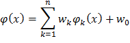
here k
is the kth radius basis function . Usually k
(1)
There are the following forms: (2)
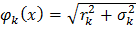

In fact, people often give k
(3)
(4)
in form (2) and within the key framework
This thesis only considers k
in form (2).
N
u 2
i
i1
Note that here we use the norm ||.|| which is the Euclidean norm u ;
vk is the center of each basis function of radius k ; k
is the radius or also known as the degree parameter
width of k .
We see that with the radius function form chosen above, the distance between the vector in
put x and center vk
The larger the value of the radius function, the smaller the value. For each k , the value
of radius k is used to control the influence domain of the radius function k .
Accordingly, if
x vk
3k then the value of function k (x)
< e9 is very small, meaningless.
Figure 10: Illustration of the influence of the radius function
For example, in the figure above a large circle represents a radial basis function, which only affects points within its radius.
Substituting formula (2) into (1) we get the mathematical representation of the radial basis function technique as follows:
(x
N
j
) �wkk (x
k 1
N
j
) w0 �wk e
k 1
xj vk 2 2
k
w0 y
(5)
j
A very advantageous feature when using the radius function to solve problems
multivariate interpolation, that is when considering the squared error
n
E
i1
xi yi 2
then
kk
It has been proven that E has only one extreme value. Therefore, finding the parameters of the radial basis functions (w, vk, ) so that E reaches its minimum will be
very fast and effective solution
1.3.2 RBF Neural Network Architecture
RBF network is a type of feedforward artificial neural network consisting of three layers.
It consists of n nodes of the input layer for the input vector
x Rn , N hidden neurons (values
of the kth hidden neuron is the return value of the radius basis function k ) and m output neurons.
x
i
k
w
i
w
0
w
0
INPUT
OUTPUT
Y
X
HIDDEN
Figure 11: Architecture of RBF network
Of course, as mentioned above, without losing generality, the content of this thesis only considers the case m=1.
1.3.3 Training characteristics of RBF Neural Network
The advantages of RBF networks are short training time, very fast and simple setup. Nowadays RBF Neural Networks are used in many fields:
Image processing
Speech Recognition Digital Signal Processing
Targeting for Medical Diagnostic Radar
Pattern Recognition Error Detection Process
….
CHAPTER 2:
RBF NETWORK TRAINING ITERATIVE ALGORITHM
The contents of this chapter include:
2.1 Describe the two-phase HDH iteration algorithm for arbitrary training data
2.2 Description of the single-phase HDH iteration algorithm used for evenly spaced training data (details of these two algorithms can be found in [6])
2.1. TWO-PHASE ITERATIVE ALGORITHM FOR TRAINING RBF NETWORK
In this chapter, before mentioning the iterative algorithm, I would like to present the theoretical basis used to build the algorithm.
2.1.1 Simple iteration method to solve linear equation system
Suppose we need to solve the system of equations
Ax=B
First we convert to equivalent system
X=Bx+d In which B is a square matrix of order n satisfying j

||B||=max{  i,j| / i=1..n} Single iteration method
For any vector x0=, the sequence of solutions of the equation is constructed by
iterative formula

satisfy
With error estimates
xk+1 = Bxk + d; (  i,jxkj+d)
= x* where x* is the only correct solution of

||x*iski|| <= max{| xkj – xk1j |}
Usually we can choose x0=d, then we consider that we have calculated the initial approximation with x0 = 0 and x0=d is the next step.
2.1.2 Two-phase iterative algorithm for training RBF network
Consider the training set xk , yk N
k 1
;xk �Rn , yk �Rm , without loss of generality,
Here we consider the RBF network with one output neuron ( m = 1 ), then the mathematical representation of the RBF network is:
( x i )
N
0
k 1
wkk
( x i ) w
yes
(1)
Consider the matrix
where (xi ) e||x x || / k , note that here
ik 2 2
k,i NN
k ,ik
We choose the center of the radial basis functions to be all points in the input data set X.
We denote I as the unit matrix of order N ; W = N -dimensional space R N in which:
w1
...
wN
, Z =
z1
...
zN
are the vectors in

and put
I
,
k , j
k N
NxN
(2)
(3)
then
0; when : k j
jk 2 2
(4)
k , j
e||x x || / k ; when : kj
Then the system of equations (1) is equivalent to the system:
W= W +Z (5)
As stated in 1.3.1, with arbitrary chosen parameters k and w0, system (1) and therefore system
(5) always has a unique solution W. Later the value w0 is chosen as the average of the yk values:
0
w =1 N yk
N k 1
(6)
For each k
N, we have the function qk of
k is determined as follows:
N
qk k , j
j 1
(7)
The function qk is monotonically increasing and for every positive number q < 1 there always exists a value k such that
let qk( k )=q.
2.1.3. Algorithm description.
Given the error and positive constants q, <1, the algorithm consists of 2
phase to determine the parameters k and W*. In the first phase, we will determine the k to
qk q and closest to q (that is, if k=k/ then qk>q). The next phase finds the solution
approximate W* of (5) by a simple iterative method. The algorithm is specified
in figure 12.
Proceduce 2-phase algorithm to train RBF network for k=1 to N do
Determine the k so that qk q, and if k=k/ then qk>q; // Phase 1
Find W* by simple iteration method (or Seidel iteration method); //Phase 2
End
Figure 12: HDH algorithm for training RBF network
To find the solution W* of system (5), we perform the following iterative procedure. Initialize W0=Z ;
Calculate
Wk+1=
Wk +Z ; (8)
If the termination condition is not satisfied, assign W0 := W1 and return to step 2;
N
For each N-dimensional vector u, we denote the norm u *
Choose one of the following expressions. a)
uj , the termination condition can be
j 1
q
1 q
W 1 W 0
*
b)
Z *
ln (1 q )
ln
t in q
ln Z *
ln q
ln(1
q) , where t is the number of iterations.
(9)
(10)
2.1.4. Comments
This algorithm has the advantage of being very simple to set up and very fast convergence speed and we can adjust the interpolation error value to be arbitrarily small. However, due to the complex network architecture
complex, so the phenomenon of overfitting often occurs for the training data set. To understand more about the HDH algorithm (see more at [6]). There, the author, with experimental research results, showed that the calculation speed and generality of the two-phase HDH iteration algorithm are much better than other classic algorithms such as the Gradient iteration method or the QTL algorithm ..... For brevity and to distinguish it from the one-phase iteration algorithm that will be presented right after, we call this two-phase HDH iteration algorithm the HDH2 algorithm.
2.2 ONE-PHASE ITERATIONAL ALGORITHM FOR TRAINING RBF NETWORKS WITH EQUALLY SPACED DATASETS
The above two-phase iteration algorithm has the characteristic that the training time of phase one occupies the majority. In the case of equally spaced training milestones, the two-phase iteration algorithm can omit this first phase, becoming a single-phase algorithm. This algorithm trains on equally spaced milestones and is often applied to applications in the field of
computer graphics, pattern recognition, engineering problems
technique…. and is the basis
basis
prize
Solve the interpolation problem with the next chapter dataset.
whether training noise is to be presented in
2.2.1 Representation of interpolation landmarks
The interpolation points are equidistant points, which can be represented as xi1,i2…,in =  ,…,
,…,  )
)

in which x =  + ik.hk . With k representing the direction, hk (k=1,2,..,n) is a constant representing the distance between 2 equidistant landmarks of 1 direction, representing the change of direction xk ; ik takes values from 0 to nk ; with nk+1 being the number of landmarks divided by each direction
2.2.2. Algorithm description:
Instead of the Euclidean norm, we consider the Mahalanobis norm: ||x|| = xT Ax, where A is a matrix of the form
The parameter  k will be chosen = hk . Then, expression (1) in section 2.1.2 can be rewritten as the following formula:

 (x) =
(x) =  i1..in(x)+w0
Matrix
become:

=
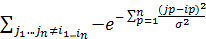
qi1..in can be rewritten as qi1..in =
Applying some mathematical transformations, see details in [6], the author has
Prove that for radius  i1..in to satisfy the condition qi1..in < q then:
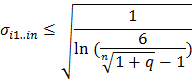
So, we can choose
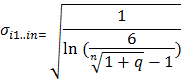
for all radius functions to ensure that the stopping condition always occurs. Thus, the initial phase of calculating the width parameter for each radius function, which takes up most of the training time, is solved immediately, the two-phase iteration problem becomes a single-phase iteration algorithm for training on equidistant landmarks.
2.2.3. Comments
According to the experimental results in [6], along with showing that the two-phase HDH iteration algorithm has shown good generality and much faster training time than other algorithms, also in [6], with the experimental results the author also pointed out that this one-phase HDH iteration algorithm with a large reduction in training time has shown a great advantage in calculation speed, in addition to showing that the generality of the one-phase HDH iteration algorithm is even better than the two-phase HDH iteration algorithm.
This algorithm has the characteristic that for a given value domain, the more densely spaced the landmarks are, the better the generality.