Understanding spectral subtraction algorithms in speech processing - 2

INTRODUCTION

Speech plays a very important role in communication. The process of transmitting speech signals through media is affected by interference, so the quality is reduced. Along with speech is the appearance of many types of voice services like today. However, preserving speech signals on these services is extremely difficult due to signal loss and degradation, and especially the impact of interference will make the speech signal no longer the same as the original. Therefore, Speech Enhancement algorithms were born. Although it is impossible to preserve the original signal, using these algorithms, we can enhance the quality of speech and reduce background noise so that the signal after processing to the listener still carries full information content and does not cause discomfort to the listener due to interference. Therefore, Speech Enhancement plays a very important role in the field of speech.

In this project, we will study the spectrum subtraction algorithm in speech processing. The algorithm is based on the principle of recognizing the presence of noise and can achieve the goal of estimating the spectrum of the voice by subtracting the spectrum of the noise from the spectrum of the noisy voice. We will analyze each part according to the development of the algorithm and evaluate the results that the algorithm brings.

To carry out the content, my project is structured into 4 chapters:

Maybe you are interested!

Chapter 1: Overview of Speech Enhancement : This chapter introduces some basic concepts of digital signals, transformations, understanding of noise types, speech signals and speech formation. In addition, it also introduces an overview of some algorithms in Speech Enhancement.

Chapter 2 : Speech Quality Evaluation : This chapter introduces several different evaluation methods used to evaluate the performance of speech enhancement algorithms.

Chapter 3: Spectral Subtraction Algorithm: This chapter delves into the fundamentals of the algorithm.

Chapter 4: Simulation using matlap software : This chapter simulates using matlap software to reduce noise of speech signal using the algorithm studied in chapter 3, from which comments and evaluations are given.

The research method of the project is to study the theory of algorithms to build flowcharts of algorithms, perform speech processing using those algorithms. Based on the results achieved, then use objective evaluation methods to evaluate the effectiveness of the processing algorithm in a real environment.

CHAPTER 1: OVERVIEW OF SPEECH QUALITY IMPROVEMENT

1.1 Chapter Introduction

The chapter covers the purpose of speech enhancement, types of noise in speech, how speech is formed, and characteristics of speech signals. The chapter also provides an overview of algorithms used in speech enhancement.

1.2 What is voice quality enhancement?

Speech enhancement is concerned with improving the perception of speech that has been degraded by the presence of noise in the speech. In most applications, the goal of speech enhancement is to improve the quality and intelligibility of speech that has been degraded by noise. The improvement in quality is good because it reduces the difficulty for the listener to listen and in many cases it also helps the listener to listen in environments with high levels of noise that persist for a long time. Speech enhancement algorithms reduce and compress background noise to some extent and are referred to as noise compression algorithms.

In many cases, the need for enhancement in speech signals arises when speech signals are formed in noisy areas or are affected by noise in communication channels. There are many scenarios that require Speech enhancement in various cases, for example, for voice information, on cellular telephone systems, which are affected by background noise from cars, restaurants, etc. when transmitting to the destination. Therefore, algorithms in speech enhancement can be used to improve the quality of speech at the receiving point, on the other hand, it can be used in the preprocessing blocks of speech coding systems used in standard cellular telephones. In speech recognition, noisy speech is preprocessed by quality enhancement algorithms before being recognized. In aviation communications, speech enhancement techniques need to be used to improve the quality and intelligibility of pilot speech affected by noise in the cockpit. Therefore, improving the voice quality is also very necessary in military communications. In a voice conference system, if a noise source appears in a certain area, it will be transmitted to all other areas. Algorithms to improve the quality of

Voice quality is used as preprocessing or noise cleaning in the voice before amplification.

As the examples above illustrate, the goals of enhancement algorithms depend on the application. Ideally, we would like Speech enhancement to improve both the quality and intelligibility or transparency of speech. However, in practice, Speech enhancement algorithms can only improve the quality of speech. It can reduce background noise in speech but it will increase the distortion of the speech signal, which reduces the intelligibility of speech. Therefore, the main requirement in designing a Speech enhancement algorithm is to ensure that noise is compressed and that there is no distortion in the perception of the speech signal.

The general solution to speech enhancement problems depends largely on the application, such as the source of noise and interference, the relationship between noise and the clean signal, and the number of microphones and sensors available. Interference can be viewed as noise or as a speech signal, depending on the environment, it can be viewed as a contention between speakers. Noise characteristics can be added to the clean signal if the sound is generated in a reverberant room. Furthermore, noise can be statistically correlated or uncorrelated with the clean signal. The number of microphones can also affect the effectiveness of speech enhancement algorithms.

1.3 Signals, systems and signal processing

1.3.1 Signal

A signal is a physical quantity that carries information. Mathematically, a signal can be described as a function of time, space, or other independent variables. For example, the function: x(t) = 20t 2 describes a signal that varies with time.

t. Or another example, the function: s(x,y) = 3x + 5xy + y 2 describes the signal as a function of two variables

independent x and y, where x and y represent two coordinates in the plane.

The two signals in the above example of the signal class are represented exactly as functions of the independent variables. However, in reality, the relationships between physical quantities and independent variables are often very complex, so it is not possible to represent the signals as in the two examples above.

Figure 1.1 Speech signal.

Take speech signal as an example – it is the variation of air pressure over time. For example, when we pronounce the word “away”, its waveform is shown as in the figure above.

1.3.2 Signal source

All signals are produced by some source, in some way. For example, a speech signal is produced by forcing air through the vocal cords. A photograph is produced by exposing a photographic film to some scene/object. Such signal production usually involves a system, which responds to some stimulus. In a speech signal, the system is the articulatory system, consisting of the lips, teeth, tongue, vocal cords, etc. The stimulus associated with the system is called the signal source. Thus, we have speech sources, photographic sources, and other signal sources.

1.3.3 Systems and signal processing

A system is a physical device that performs some action on a signal. For example, a filter used to reduce noise in a message-carrying signal is called a system. When we pass a signal through a system, such as a filter, we say that we have processed the signal. In this context, signal processing involves filtering noise from the desired signal.

Signal processing refers to a series of tasks or operations performed on signals to achieve some purpose, such as extracting information contained within the signal or transmitting a signal carrying information from one place to another.

Here we need to pay attention to the definition of system, it is not only physical equipment but also signal processing software or a combination of hardware and software.

software. For example, when processing digital signals using logic circuits, the processing system here is the hardware. When processing with a digital computer, the action on the signal includes a series of operations performed by a software program. When processing with microprocessors-the system includes a combination of hardware and software, each part performing certain separate tasks.

1.3.4 Signal classification

The methods we use in signal processing depend closely on the characteristics of the signal. There are specific methods that apply to a certain type of signal. Therefore, we need to first look at the classification of signals in relation to specific applications. We can classify signals into the following types:

- Multi-directional and multi-channel signals

- Continuous signal and discrete signal

- Continuous amplitude signal and discrete amplitude signal

- Deterministic signals and random signals

1.4 Theory of noise

1.4.1 Noise sources

Noise is a reality, it exists everywhere, on the streets, in cars, in offices, in restaurants, in buildings. It can be the sound of cars on the road, the noise on construction sites, the noise from the fans running in PCs, the ringing of phones…, it exists in different shapes and forms in our daily lives.

Noise can be located in a fixed location and not change over time, such as the noise from a PC fan. Noise can also be non-stationary, such as restaurant noise, which is the sound of many people talking mixed in various ways with the noise from the kitchen. The spectral and temporal characteristics of restaurant noise vary irregularly, so noise suppression in environments with such variable noise is much more difficult than noise sources that are static.

The special characteristics of these types of noise are the shape of the spectrum and the distribution of noise energy in the frequency domain. For example, noise caused by wind has its energy concentrated at low frequencies below 500Hz. But for noise in restaurants, cars, and trains, it is different, its energy is distributed over a wide frequency range.

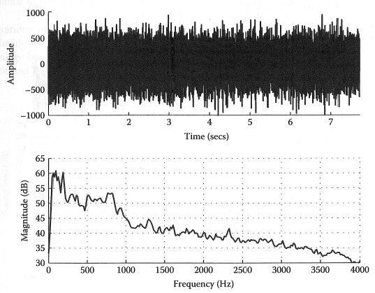
Figure 1.2 Shape and distribution of average noise energy spectrum on the vehicle.

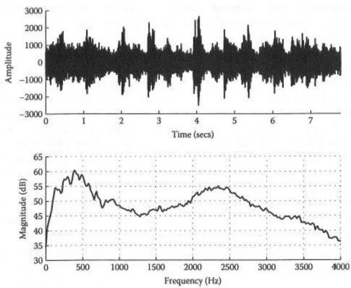
Figure 1.3 Shape and average power spectrum distribution of shipboard noise.

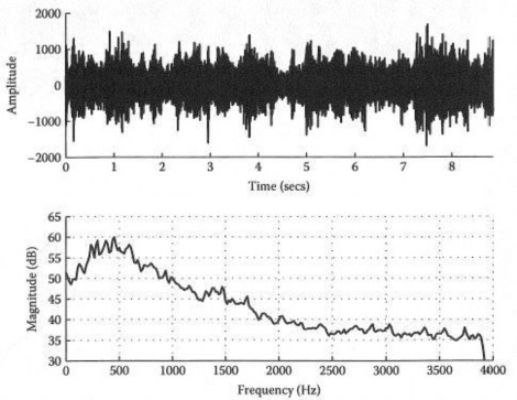
Figure 1.4 Shape and average power spectrum distribution of noise in a restaurant.

1.4.2 Noise and speech signal levels in different environments

The critical point in designing Speech enhancement algorithms is to recognize the range of speech and noise intensity levels in real-world environments. From this, we can describe the range of signal-to-noise ratio (SNR) levels encountered in real-world environments. This is important to evaluate the effectiveness of Speech enhancement algorithms in suppressing noise and improving speech quality over the range of SNR levels.

The level of speech and noise is measured by sound level. The measurement here is the sound pressure level measured in dB SPL (sound pressure level). The distance between the speaker and the listener also affects the sound intensity level, it corresponds to the measurement taken when the microphone is placed at different distances. The typical distance in face-to-face communication is 1m, when that distance is doubled, the sound intensity level decreases by 6 dB.

The figure below shows the average sound levels between speech and noise in different environments. The lowest levels of noise are found in environments such as classrooms, homes, hospitals, and buildings. In different environments, the sound levels of noise range from 50 to 55 dB SPL, and the sound levels of speech range from 60 to 70 dB SPL. And the recommendation is to

It turns out that the effective SNR level in these environments is 5 to 15 dB. The noise level is very high in subway environments, on airplanes, it reaches about 70 to 75 dB SPL. And the speech level in these environments is also at that level, so the SNR level in these environments is almost 0 dB.

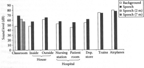
Figure 1.5 Noise and speech levels (measured in SPL dB) in different environments.

1.5 Discrete-time signals

A discrete-time signal x(n) can be generated by sampling a continuous-time signal x a (t) with a sampling period T s (sampling frequency F s = 1/ T). We have

x a (t)| t=nT = x a (nT) = x(n) , -∞ < n< ∞ (1.1)

Note that n is an integer variable, x(n) is a function of the integer variable, specified at integer values n. When n is not an integer, then x(n) is undefined, not zero. In many books on digital signal processing, it is a convention: when the variable is an integer, the variable is placed in square brackets and when the variable is continuous, it is placed in round brackets. From here on, we denote the discrete signal as: x[n].

Some basic discrete signals

1.5.1 Unit step signal

u[n] =

 1, n  0



 2, n  0

(1.2)

The displacement jump signal has the following form:

u[n - n o ] =

 1,



 0,