RELATIONSHIP BETWEEN EBIT AND EPS (6)
Indifference point = Total assets x Interest payable
If EBIT is lower than the indifference point => Equity financing generates higher EPS than debt financing
If EBIT exceeds the indifference point => Option
FINANCIAL LEVERAGE (1)
- Financial leverage measures the extent to which a company uses debt.
- Degree of Financial Leverage (DFL) measures the change in EPS in response to a change in EBIT.
Debt financing yields higher EPS than equity financing
DFL
EPS / EPS
EBIT / EBIT
(9.6)
21 22
FINANCIAL LEVERAGE (2)
- DFL in case the capital structure includes common stock, debt and preferred stock.
FINANCIAL LEVERAGE (3)
- DFL of preferential stock financing plan.
DFL EBIT (9.7)
EBIT I PD /(1 t )
DFL 2,700,000
2,700,000
2,700,000 550,000 /(1 0.4)
1.51
- DFL in case the capital structure consists of common stock and debt.
- DFL of debt financing option.
DFL EBIT (9.8)
EBIT I
DFL
2,700,000
2,700,000
2,700,000 600,000
1.29
23 24
TOTAL LEVERAGE - DTL (1)
Combined leverage measures the impact of changes in sales or output on EPS.
DTL DOLxDFL
(9.9)
DTL
Q
DTL
S
Q ( P V )
Q ( P V ) F I PD /(1 t )
EBIT F
EBIT I PD /(1 t )
(9.10)
(9.11)
25
Fulbright Economics Teaching Program Financial Analysis Lecture 8 Academic Year 2006-2007 Lecture
OPERATING LEVERAGE AND FINANCIAL LEVERAGE
In mechanics, we are familiar with the concept of leverage as a tool to amplify force to turn a small force into a larger force acting on the object we need to move. In business, people borrow the term “leverage” to refer to the use of fixed costs to increase the profitability of the company. In this article, we will explore the principles of using leverage in business, including operating leverage and financial leverage.
1. Operating leverage
1.1 Analysis of the impact of operating leverage
Operating leverage is the extent to which a company uses fixed operating costs. Here we only analyze the short run because in the long run all costs are variable.
Fixed costs are costs that do not change when volume changes. Fixed costs can include things like depreciation, insurance, a portion of utility costs, and a portion of administrative costs.
Variable costs are costs that change when quantity changes, such as raw materials costs, direct labor, a portion of utilities, sales commissions, and a portion of administrative costs.
In business, we invest fixed costs in the hope that sales volume will generate enough revenue to cover both fixed and variable costs. Like a lever in mechanics, the presence of fixed operating costs causes changes in sales volume to magnify changes in profit (or loss). To illustrate this, consider the example given in Table 8.1 on page 2.
The results of the analysis of the impact of operating leverage are shown in Part B. For each company, revenue and variable costs increased by 50% while fixed costs remained unchanged. All companies showed the impact of operating leverage, which was shown in that revenue increased by only 50% but profits increased at a greater rate, namely 400, 100 and 330% for companies F, V and company 2F, respectively.
Table 8.1 : Effect of operating leverage on profits
Company F | Company V | 2F Company | |
Part A : Before changing revenue | |||
Revenue | 10,000$ | 11,000$ | 19,500$ |
Operating costs | |||
Fixed costs | 7,000 | 2,000 | 14,000 |
Variable costs | 2,000 | 7,000 | 3,000 |
Operating profit (EBIT) | 1,000 | 2,000 | 2,500 |
Operating leverage ratio | |||
Fixed cost/total cost | 0.78 | 0.22 | 0.82 |
Fixed cost/revenue | 0.70 | 0.18 | 0.72 |
Part B : After revenue increases by 50% in the following years | |||
Revenue | 15,000$ | 16,500$ | 29,250$ |
Operating costs | |||
Fixed costs | 7,000 | 2,000 | 14,000 |
Maybe you are interested!
-
![Pre-tax Profit of Bidv Tien Giang in the Period 2011-2015
zt2i3t4l5ee
zt2a3gsnon-credit services, joint stock commercial bank
zt2a3ge
zc2o3n4t5e6n7ts
At that time, the Branch had to set aside a provision for credit risks, which reduced the Branchs income.
Chart 2.2. Pre-tax profit of BIDV Tien Giang in the period 2011-2015
Unit: Billion VND
140
120
100
80
60
40
20
0
63.3
80.34
89.29
110.08
131.99
2011 2012 2013 2014 2015
Profit before tax
(Source: Report on the implementation of the annual business plan of the General Planning Department of BIDV Tien Giang [24])
However, through chart 2.2, it can be seen that BIDV Tien Giangs profit is still increasing continuously, and its operating efficiency is currently leaking. This is a contribution of non-credit services, and this service segment will be increasingly focused on growth by BIDV Tien Giang to ensure the highest profit safety because credit activities have many potential risks. At the same time, focusing on developing non-credit services is consistent with one of the contents of restructuring the financial activities of credit institutions in the project Restructuring the system of credit institutions in the period 2011-2015 approved by the Prime Minister in Decision No. 254/QD-TTg dated March 1, 2012 [14]: Gradually shifting the business model of commercial banks towards reducing dependence on credit activities and increasing income from non-credit services.
2.2. Current status of non-credit service development at BIDV Tien Giang.
2.2.1. BIDV Tien Giang has deployed the development of non-credit services in recent times.
Along with the development of the Head Office, BIDV Tien Giangs products and services are constantly improved and deployed in a diverse manner to ensure provision for many different customer groups in the area: individual customers, corporate customers, and financial institutions. Typical services are as follows: Payment services, treasury services, guarantee services, card services, trade finance, other services: Western Union, insurance commissions, consulting services, foreign exchange derivatives trading, e-banking services,...
2.2.1.1. Payment services:
In accordance with the Prime Ministers Project to promote non-cash payments in Vietnam [15], banks in Tien Giang province have continuously developed payment services to reduce customers cash usage habits through card services and electronic banking services such as: salary payment through accounts, focusing on developing card acceptance points, developing multi-purpose cards, paying social insurance by transfer, paying bills through banks, etc.
Chart 2.3. Net income from payment services in the period 2011-2015
Unit: Million VND
6000
5000
4000
3000
2000
1000
0
3922 4065
4720 5084 5324
2011 2012 2013 2014 2015
Net income from payment services
(Source: Report on the implementation of the annual business plan of the General Planning Department of BIDV Tien Giang [24])
Along with the technological development of the entire system, BIDV Tien Giang has a payment system with a fairly stable transaction processing speed, bringing many conveniences to customers. The results of observing chart 2.3 show that the income from payment services that the Branch has achieved has grown over the years but the speed is not high and the products are not outstanding compared to other banks. Domestic payment products such as: Online bill payment, electricity bills, water bills, insurance premiums, cable TV bills, telecommunications fees, airline tickets, etc. bring many conveniences to customers. Regarding international payment, this is an indispensable activity for foreign economic activities, BIDV Tien Giang is providing international payment methods for small enterprises producing agriculture, aquatic food and seafood that have credit relationships with banks in industrial parks in Tien Giang province such as: money transfer, collection, L/C payment.
2.2.1.2. Treasury services:
BIDV Tien Giang always focuses on ensuring treasury safety and currency security, always complies with legal regulations, and minimizes risks in operations such as: counting and collecting money from customers, receiving and delivering internal transactions, collecting from the State Bank (SBV) or other credit institutions, receiving ATM funds, bundling money, etc. BIDV Tien Giangs treasury service management department is always fully equipped with modern machinery and equipment such as: money transport vehicles, fire prevention tools, money counters, money detectors, magnifying glasses, etc. to ensure absolute safety in treasury operations, immediately identifying real and fake money and other risks that may affect people and assets of the bank and customers. In addition, implementing regulation 2480/QC dated October 28, 2008 between the State Bank of Tien Giang province and the Provincial Police on coordination in the fight against counterfeit money, in the 3-year review of implementation, BIDV Tien Giang discovered, seized and submitted to the State Bank of Tien Giang province 475 banknotes of various denominations and was commended by the Provincial Police and the State Bank of Tien Giang province [17].
Chart 2.4. Net income from treasury services in the period 2011-2015
Unit: Million VND
350
300
250
200
150
100
50
0
105 122
309 289 279
2011 2012 2013 2014 2015
Net income from treasury services
(Source: Report on the implementation of the annual business plan of the General Planning Department of BIDV Tien Giang [24])
However, as shown in Figure 2.4, income from treasury operations is not high and fluctuates. Specifically, in the period 2011-2013, net income increased and increased most sharply in 2013, then in the period 2013-2015, there was a downward trend. This fluctuation is due to the fact that fees collected from treasury services are often very low and can even be waived to attract customers to use other services.
2.2.1.3. Guarantee and trade finance services:
BIDV Tien Giang, thanks to the advantages of the province and the favorable location of the Branch, has continuously focused on developing income from guarantee services and trade finance.
Chart 2.5. Net income from guarantee and trade finance services in the period 2011-2015
Unit: Million VND
14000
12000
10000
8000
6000
4000
2000
0
5193 5695
2742 3420
8889
3992
11604 12206
5143 5312
2011 2012 2013 2014 2015
Net income from guarantee services Net income from Trade Finance
(Source: Report on the implementation of the annual business plan of the General Planning Department of BIDV Tien Giang [24])
Through chart 2.5, we can see that BIDV Tien Giangs income from guarantee services and trade finance has grown over the years. The reason is: Among BIDV Tien Giangs corporate customers, the construction industry is the industry with the highest proportion of customers after the trading industry, this is a group of customers with potential to develop guarantee services. The second group of customers is corporate customers in the fields of agricultural production, livestock and seafood processing with high import and export turnover in the area.
are the target of trade finance development. In addition, BIDV Tien Giang also focuses on continuously developing these customer groups to increase revenue for many other products and services in the future.
2.2.1.4. Card and POS services:
As a service that BIDV Tien Giang has recently developed strongly, it can be said that this is a very potential market and has the ability to develop even more strongly in the future. Card services with outstanding advantages such as fast payment time, wide payment range, quite safe, effective and suitable for the integration trend and the Project to promote non-cash payments in Vietnam. Cards have become a modern and popular payment tool. BIDV Tien Giang early identified that developing card services is to expand the market to people in society, create capital mobilized from card-opened accounts, contribute to diversifying banking activities, enhance the image of the bank, bring the BIDV Tien Giang brand to people as quickly and easily as possible. BIDV Tien Giang is currently providing card types such as: credit cards (BIDV MasterCard Platinum, BIDV Visa Gold Precious, BIDV Visa Manchester United, BIDV Visa Classic), international debit cards (BIDV Ready Card, BIDV Manu Debit Card), domestic debit cards (BIDV Harmony Card, BIDV eTrans Card, BIDV Moving Card, BIDV-Lingo Co-branded Card, BIDV-Co.opmart Co-branded Card). These cards can be paid via POS/EDC or on the ATM system. In addition, with debit cards, customers can not only withdraw money via ATMs but also perform utilities such as mobile top-up, online payment, money transfer,... through electronic banking services.
In order to attract customers with card services, BIDV Tien Giang has continuously increased the installation of ATMs. As of December 31, 2015, BIDV Tien Giang has 23 ATMs combined with 7 ATMs in the same system of BIDV My Tho, so the number of ATMs is quite large, especially in the center of My Tho City, but is not yet fully present in the districts. Basic services on ATMs such as withdrawing money, checking balances, printing short statements,... BIDV ATMs accept cards from banks in the system.
Banknetvn and Smartlink, cards branded by international card organizations Union Pay (CUP), VISA, MasterCard and cards of banks in the Asian Payment Network. From here, cardholders can make bill payments for themselves or others at ATMs, by simply entering the subscriber number or customer code, booking code that service providers notify and make bill payments.
Chart 2.6. Net income from card services in the period 2011-2015
Unit: Million VND
3500
3000
2500
2000
1500
1000
500
0
687
1023
1547
2267
3104
2011 2012 2013 2014 2015
Net income from card services
(Source: Report on the implementation of the annual business plan of the General Planning Department of BIDV Tien Giang [24])
Through chart 2.6, it can be seen that BIDV Tien Giangs card service income is constantly growing because the Branch focuses on developing businesses operating in industrial parks, which are the source of customers for salary payment products, ATMs, BSMS. Specifically, there are companies such as Freeview, Quang Viet, Dai Thanh, which are businesses with a large number of card openings at the Branch, contributing to the increase in card service fees [25].
Table 2.6. Number of ATMs and POS machines in 2015 of some banks in Tien Giang area.
Unit: Machine
STT
Bank name
Number of ATMs
Cumulative number of ATM cards
POS machine
1
BIDV Tien Giang
23
97,095
22
2
BIDV My Tho
7
21,325
0
3
Agribank Tien Giang
29
115,743
77
4
Vietinbank Tien Giang
16
100,052
54
5
Dong A Tien Giang
26
97,536
11
6
Sacombank Tien Giang
24
88,513
27
7
Vietcombank Tien Giang
15
61,607
96
8
Vietinbank - Tay Tien Giang Branch
6
46,042
38
(Source: 2015 Banking Activity Data Report of the General and Internal Control Department of the Provincial State Bank [21])
Through table 2.6, the author finds that the number of ATMs of BIDV Tien Giang is not much, ranking fourth after Agribank Tien Giang, Dong A Tien Giang, Sacombank Tien Giang. The number of POS machines of BIDV Tien Giang is very small, only higher than Dong A Tien Giang and BIDV My Tho in the initial stages of merging the BIDV system. Besides, BIDV Tien Giang has a high number of cards increasing over the years (table 2.7) but the cumulative number of cards issued up to December 31, 2015 is still relatively low compared to Agribank, Vietcombank, Dong A (table 2.6).
div.maincontent .content_head3 { color: black; font-family:Times New Roman, serif; font-style: normal; font-weight: bold; text-decoration: none; font-size: 14pt; }
div.maincontent .p { color: black; font-family:Times New Roman, serif; font-style: normal; font-weight: normal; text-decoration: none; font-size: 14pt; margin:0pt; }
div.maincontent p { color: black; font-family:Times New Roman, serif; font-style: normal; font-weight: normal; text-decoration: none; font-size: 14pt; margin:0pt; }
div.maincontent .s1 { color: black; font-family:Courier New, monospace; font-style: normal; font-weight: normal; text-decoration: none; font-size: 14pt; }
div.maincontent .s2 { color: black; font-family:Times New Roman, serif; font-style: italic; font-weight: normal; text-decoration: none; font-size: 13pt; }
div.maincontent .s3 { color: black; font-family:Times New Roman, serif; font-style: italic; font-weight: bold; text-decoration: none; font-size: 14pt; }
div.maincontent .s4 { color: black; font-family:Times New Roman, serif; font-style: italic; font-weight: normal; text-decoration: none; font-size: 14pt; }
div.maincontent .s5 { color: black; font-family:Times New Roman, serif; font-style: normal; font-weight: normal; text-decoration: none; font-size: 14pt; }
div.maincontent .s6 { color: black; font-family:Times New Roman, serif; font-style: normal; font-weight: bold; text-decoration: none; font-size: 14pt; }
div.maincontent .s7 { color: black; font-family:Times New Roman, serif; font-style: normal; font-weight: normal; text-decoration: none; font-size: 13.5pt; }
div.maincontent .s8 { color: black; font-family:Arial, sans-serif; font-style: normal; font-weight: normal; text-decoration: none; font-size: 9pt; }
div.maincontent .s9 { color: black; font-family:Arial, sans-serif; font-style: normal; font-weight: normal; text-decoration: none; font-size: 9pt; vertical-align: -2pt; }
div.maincontent .s10 { color: black; font-family:Arial, sans-serif; font-style: normal; font-weight: normal; text-decoration: none; font-size: 9pt; vertical-align: 5pt; }
div.maincontent .s11 { color: black; font-family:Arial, sans-serif; font-style: normal; font-weight: normal; text-decoration: none; font-size: 9pt; vertical-align: -5pt; }
div.maincontent .s12 { color: black; font-family:Arial, sans-serif; font-style: normal; font-weight: normal; text-decoration: none; font-size: 9pt; vertical-align: -3pt; }
div.maincontent .s13 { color: black; font-family:Arial, sans-serif; font-style: normal; font-weight: normal; text-decoration: none; font-size: 9pt; vertical-align: -4pt; }
div.maincontent .s14 { color: black; font-family:Arial, sans-serif; font-style: normal; font-weight: normal; text-decoration: none; font-size: 7.5pt; }
div.maincontent .s15 { color: black; font-family:Times New Roman, serif; font-style: italic; font-weight: normal; text-decoration: none; font-size: 14pt; }
div.maincontent .s16 { color: black; font-family:Arial, sans-serif; font-style: normal; font-weight: normal; text-decoration: none; font-size: 10.5pt; }
div.maincontent .s17 { color: black; font-family:Arial, sans-serif; font-style: normal; font-weight: normal; text-decoration: none; font-size: 9.5pt; }
div.maincontent .s18 { color: black; font-family:Arial, sans-serif; font-style: normal; font-weight: normal; text-decoration: none; font-size: 10.5pt; vertical-align: -1pt; }
div.maincontent .s19 { color: black; font-family:Arial, sans-serif; font-style: normal; font-weight: normal; text-decoration: none; font-size: 10.5pt; vertical-align: -5pt; }
div.maincontent .s20 { color: black; font-family:Arial, sans-serif; font-style: normal; font-weight: normal; text-decoration: none; font-size: 10.5pt; vertical-align: -2pt; }
div.maincontent .s21 { color: black; font-family:Arial, sans-serif; font-style: normal; font-weight: normal; text-decoration: none; font-size: 10pt; }
div.maincontent .s22 { color: black; font-family:Calibri, sans-serif; font-style: normal; font-weight: normal; text-decoration: none; font-size: 10.5pt; }
div.maincontent .s23 { color: black; font-family:Calibri, sans-serif; font-style: normal; font-weight: normal; text-decoration: none; font-size: 10.5pt; vertical-align: -3pt; }
div.maincontent .s24 { color: black; font-family:Calibri, sans-serif; font-style: normal; font-weight: normal; text-decoration: none; font-size: 10.5pt; vertical-align: -5pt; }
div.maincontent .s25 { color: black; font-family:Times New Roman, serif; font-style: normal; font-weight: normal; text-decoration: none; font-size: 10.5pt; }
div.maincontent .s26 { color: black; font-family:Calibri, sans-serif; font-style: normal; font-weight: normal; text-decoration: none; font-size: 10.5pt; vertical-align: -4pt; }
div.maincontent .s27 { color: black; font-family:Calibri, sans-serif; font-style: normal; font-weight: normal; text-decoration: none; font-size: 10.5pt; vertical-align: -6pt; }
div.maincontent .s28 { color: black; font-family:Calibri, sans-serif; font-style: normal; font-weight: normal; text-decoration: none; font-size: 10.5pt; vertical-align: -1pt; }
div.maincontent .s29 { color: black; font-family:Calibri, sans-serif; font-style: normal; font-weight: normal; text-decoration: none; font-size: 11.5pt; }
div.maincontent .s30 { color: black; font-family:Calibri, sans-serif; font-style: normal; font-weight: normal; text-decoration: none; font-size: 11pt; }
div.maincontent .s31 { color: black; font-family:Times New Roman, serif; font-style: normal; font-weight: normal; text-decoration: none; font-size: 11pt; }
div.maincontent .s32 { color: black; font-family:.VnTime, sans-serif; font-style: normal; font-weight: normal; text-decoration: none; font-size: 14pt; }
div.maincontent .s33 { color: black; font-family:Cambria, serif; font-style: normal; font-weight: normal; text-decoration: none; font-size: 10.5pt; }
div.maincontent .s34 { color: black; font-family:Cambria, serif; font-style: normal; font-weight: normal; text-decoration: none; font-size: 10.5pt; vertical-align: -4pt; }
div.maincontent .s35 { color: black; font-family:Arial, sans-serif; font-style: normal; font-weight: normal; text-decoration: none; font-size: 11.5pt; }
div.maincontent .s36 { color: black; font-family:Arial, sans-serif; font-style: normal; font-weight: bold; text-decoration: none; font-size: 14pt; }
div.maincontent .s37 { color: black; font-family:Times New Roman, serif; font-style: normal; font-weight: bold; text-decoration: none; font-size: 13pt; }
div.maincontent .s38 { color: black; font-family:Times New Roman, serif; font-style: normal; font-weight: normal; text-decoration: none; font-size: 13pt; }
div.maincontent .s39 { color: black; font-family:Times New Roman, serif; font-style: normal; font-weight: normal; text-decoration: none; font-size: 15pt; }
div.maincontent .s40 { color: black; font-family:Times New Roman, serif; font-style: normal; fo](https://tailieuthamkhao.com/uploads/2022/06/06/dich-vu-phi-tin-dung-tai-ngan-hang-thuong-mai-co-phan-dau-tu-va-phat-8-1-120x90.png)
![Pre-tax Profit of Bidv Tien Giang in the Period 2011-2015
zt2i3t4l5ee
zt2a3gsnon-credit services, joint stock commercial bank
zt2a3ge
zc2o3n4t5e6n7ts
At that time, the Branch had to set aside a provision for credit risks, which reduced the Branchs income.
Chart 2.2. Pre-tax profit of BIDV Tien Giang in the period 2011-2015
Unit: Billion VND
140
120
100
80
60
40
20
0
63.3
80.34
89.29
110.08
131.99
2011 2012 2013 2014 2015
Profit before tax
(Source: Report on the implementation of the annual business plan of the General Planning Department of BIDV Tien Giang [24])
However, through chart 2.2, it can be seen that BIDV Tien Giangs profit is still increasing continuously, and its operating efficiency is currently leaking. This is a contribution of non-credit services, and this service segment will be increasingly focused on growth by BIDV Tien Giang to ensure the highest profit safety because credit activities have many potential risks. At the same time, focusing on developing non-credit services is consistent with one of the contents of restructuring the financial activities of credit institutions in the project Restructuring the system of credit institutions in the period 2011-2015 approved by the Prime Minister in Decision No. 254/QD-TTg dated March 1, 2012 [14]: Gradually shifting the business model of commercial banks towards reducing dependence on credit activities and increasing income from non-credit services.
2.2. Current status of non-credit service development at BIDV Tien Giang.
2.2.1. BIDV Tien Giang has deployed the development of non-credit services in recent times.
Along with the development of the Head Office, BIDV Tien Giangs products and services are constantly improved and deployed in a diverse manner to ensure provision for many different customer groups in the area: individual customers, corporate customers, and financial institutions. Typical services are as follows: Payment services, treasury services, guarantee services, card services, trade finance, other services: Western Union, insurance commissions, consulting services, foreign exchange derivatives trading, e-banking services,...
2.2.1.1. Payment services:
In accordance with the Prime Ministers Project to promote non-cash payments in Vietnam [15], banks in Tien Giang province have continuously developed payment services to reduce customers cash usage habits through card services and electronic banking services such as: salary payment through accounts, focusing on developing card acceptance points, developing multi-purpose cards, paying social insurance by transfer, paying bills through banks, etc.
Chart 2.3. Net income from payment services in the period 2011-2015
Unit: Million VND
6000
5000
4000
3000
2000
1000
0
3922 4065
4720 5084 5324
2011 2012 2013 2014 2015
Net income from payment services
(Source: Report on the implementation of the annual business plan of the General Planning Department of BIDV Tien Giang [24])
Along with the technological development of the entire system, BIDV Tien Giang has a payment system with a fairly stable transaction processing speed, bringing many conveniences to customers. The results of observing chart 2.3 show that the income from payment services that the Branch has achieved has grown over the years but the speed is not high and the products are not outstanding compared to other banks. Domestic payment products such as: Online bill payment, electricity bills, water bills, insurance premiums, cable TV bills, telecommunications fees, airline tickets, etc. bring many conveniences to customers. Regarding international payment, this is an indispensable activity for foreign economic activities, BIDV Tien Giang is providing international payment methods for small enterprises producing agriculture, aquatic food and seafood that have credit relationships with banks in industrial parks in Tien Giang province such as: money transfer, collection, L/C payment.
2.2.1.2. Treasury services:
BIDV Tien Giang always focuses on ensuring treasury safety and currency security, always complies with legal regulations, and minimizes risks in operations such as: counting and collecting money from customers, receiving and delivering internal transactions, collecting from the State Bank (SBV) or other credit institutions, receiving ATM funds, bundling money, etc. BIDV Tien Giangs treasury service management department is always fully equipped with modern machinery and equipment such as: money transport vehicles, fire prevention tools, money counters, money detectors, magnifying glasses, etc. to ensure absolute safety in treasury operations, immediately identifying real and fake money and other risks that may affect people and assets of the bank and customers. In addition, implementing regulation 2480/QC dated October 28, 2008 between the State Bank of Tien Giang province and the Provincial Police on coordination in the fight against counterfeit money, in the 3-year review of implementation, BIDV Tien Giang discovered, seized and submitted to the State Bank of Tien Giang province 475 banknotes of various denominations and was commended by the Provincial Police and the State Bank of Tien Giang province [17].
Chart 2.4. Net income from treasury services in the period 2011-2015
Unit: Million VND
350
300
250
200
150
100
50
0
105 122
309 289 279
2011 2012 2013 2014 2015
Net income from treasury services
(Source: Report on the implementation of the annual business plan of the General Planning Department of BIDV Tien Giang [24])
However, as shown in Figure 2.4, income from treasury operations is not high and fluctuates. Specifically, in the period 2011-2013, net income increased and increased most sharply in 2013, then in the period 2013-2015, there was a downward trend. This fluctuation is due to the fact that fees collected from treasury services are often very low and can even be waived to attract customers to use other services.
2.2.1.3. Guarantee and trade finance services:
BIDV Tien Giang, thanks to the advantages of the province and the favorable location of the Branch, has continuously focused on developing income from guarantee services and trade finance.
Chart 2.5. Net income from guarantee and trade finance services in the period 2011-2015
Unit: Million VND
14000
12000
10000
8000
6000
4000
2000
0
5193 5695
2742 3420
8889
3992
11604 12206
5143 5312
2011 2012 2013 2014 2015
Net income from guarantee services Net income from Trade Finance
(Source: Report on the implementation of the annual business plan of the General Planning Department of BIDV Tien Giang [24])
Through chart 2.5, we can see that BIDV Tien Giangs income from guarantee services and trade finance has grown over the years. The reason is: Among BIDV Tien Giangs corporate customers, the construction industry is the industry with the highest proportion of customers after the trading industry, this is a group of customers with potential to develop guarantee services. The second group of customers is corporate customers in the fields of agricultural production, livestock and seafood processing with high import and export turnover in the area.
are the target of trade finance development. In addition, BIDV Tien Giang also focuses on continuously developing these customer groups to increase revenue for many other products and services in the future.
2.2.1.4. Card and POS services:
As a service that BIDV Tien Giang has recently developed strongly, it can be said that this is a very potential market and has the ability to develop even more strongly in the future. Card services with outstanding advantages such as fast payment time, wide payment range, quite safe, effective and suitable for the integration trend and the Project to promote non-cash payments in Vietnam. Cards have become a modern and popular payment tool. BIDV Tien Giang early identified that developing card services is to expand the market to people in society, create capital mobilized from card-opened accounts, contribute to diversifying banking activities, enhance the image of the bank, bring the BIDV Tien Giang brand to people as quickly and easily as possible. BIDV Tien Giang is currently providing card types such as: credit cards (BIDV MasterCard Platinum, BIDV Visa Gold Precious, BIDV Visa Manchester United, BIDV Visa Classic), international debit cards (BIDV Ready Card, BIDV Manu Debit Card), domestic debit cards (BIDV Harmony Card, BIDV eTrans Card, BIDV Moving Card, BIDV-Lingo Co-branded Card, BIDV-Co.opmart Co-branded Card). These cards can be paid via POS/EDC or on the ATM system. In addition, with debit cards, customers can not only withdraw money via ATMs but also perform utilities such as mobile top-up, online payment, money transfer,... through electronic banking services.
In order to attract customers with card services, BIDV Tien Giang has continuously increased the installation of ATMs. As of December 31, 2015, BIDV Tien Giang has 23 ATMs combined with 7 ATMs in the same system of BIDV My Tho, so the number of ATMs is quite large, especially in the center of My Tho City, but is not yet fully present in the districts. Basic services on ATMs such as withdrawing money, checking balances, printing short statements,... BIDV ATMs accept cards from banks in the system.
Banknetvn and Smartlink, cards branded by international card organizations Union Pay (CUP), VISA, MasterCard and cards of banks in the Asian Payment Network. From here, cardholders can make bill payments for themselves or others at ATMs, by simply entering the subscriber number or customer code, booking code that service providers notify and make bill payments.
Chart 2.6. Net income from card services in the period 2011-2015
Unit: Million VND
3500
3000
2500
2000
1500
1000
500
0
687
1023
1547
2267
3104
2011 2012 2013 2014 2015
Net income from card services
(Source: Report on the implementation of the annual business plan of the General Planning Department of BIDV Tien Giang [24])
Through chart 2.6, it can be seen that BIDV Tien Giangs card service income is constantly growing because the Branch focuses on developing businesses operating in industrial parks, which are the source of customers for salary payment products, ATMs, BSMS. Specifically, there are companies such as Freeview, Quang Viet, Dai Thanh, which are businesses with a large number of card openings at the Branch, contributing to the increase in card service fees [25].
Table 2.6. Number of ATMs and POS machines in 2015 of some banks in Tien Giang area.
Unit: Machine
STT
Bank name
Number of ATMs
Cumulative number of ATM cards
POS machine
1
BIDV Tien Giang
23
97,095
22
2
BIDV My Tho
7
21,325
0
3
Agribank Tien Giang
29
115,743
77
4
Vietinbank Tien Giang
16
100,052
54
5
Dong A Tien Giang
26
97,536
11
6
Sacombank Tien Giang
24
88,513
27
7
Vietcombank Tien Giang
15
61,607
96
8
Vietinbank - Tay Tien Giang Branch
6
46,042
38
(Source: 2015 Banking Activity Data Report of the General and Internal Control Department of the Provincial State Bank [21])
Through table 2.6, the author finds that the number of ATMs of BIDV Tien Giang is not much, ranking fourth after Agribank Tien Giang, Dong A Tien Giang, Sacombank Tien Giang. The number of POS machines of BIDV Tien Giang is very small, only higher than Dong A Tien Giang and BIDV My Tho in the initial stages of merging the BIDV system. Besides, BIDV Tien Giang has a high number of cards increasing over the years (table 2.7) but the cumulative number of cards issued up to December 31, 2015 is still relatively low compared to Agribank, Vietcombank, Dong A (table 2.6).
div.maincontent .content_head3 { color: black; font-family:Times New Roman, serif; font-style: normal; font-weight: bold; text-decoration: none; font-size: 14pt; }
div.maincontent .p { color: black; font-family:Times New Roman, serif; font-style: normal; font-weight: normal; text-decoration: none; font-size: 14pt; margin:0pt; }
div.maincontent p { color: black; font-family:Times New Roman, serif; font-style: normal; font-weight: normal; text-decoration: none; font-size: 14pt; margin:0pt; }
div.maincontent .s1 { color: black; font-family:Courier New, monospace; font-style: normal; font-weight: normal; text-decoration: none; font-size: 14pt; }
div.maincontent .s2 { color: black; font-family:Times New Roman, serif; font-style: italic; font-weight: normal; text-decoration: none; font-size: 13pt; }
div.maincontent .s3 { color: black; font-family:Times New Roman, serif; font-style: italic; font-weight: bold; text-decoration: none; font-size: 14pt; }
div.maincontent .s4 { color: black; font-family:Times New Roman, serif; font-style: italic; font-weight: normal; text-decoration: none; font-size: 14pt; }
div.maincontent .s5 { color: black; font-family:Times New Roman, serif; font-style: normal; font-weight: normal; text-decoration: none; font-size: 14pt; }
div.maincontent .s6 { color: black; font-family:Times New Roman, serif; font-style: normal; font-weight: bold; text-decoration: none; font-size: 14pt; }
div.maincontent .s7 { color: black; font-family:Times New Roman, serif; font-style: normal; font-weight: normal; text-decoration: none; font-size: 13.5pt; }
div.maincontent .s8 { color: black; font-family:Arial, sans-serif; font-style: normal; font-weight: normal; text-decoration: none; font-size: 9pt; }
div.maincontent .s9 { color: black; font-family:Arial, sans-serif; font-style: normal; font-weight: normal; text-decoration: none; font-size: 9pt; vertical-align: -2pt; }
div.maincontent .s10 { color: black; font-family:Arial, sans-serif; font-style: normal; font-weight: normal; text-decoration: none; font-size: 9pt; vertical-align: 5pt; }
div.maincontent .s11 { color: black; font-family:Arial, sans-serif; font-style: normal; font-weight: normal; text-decoration: none; font-size: 9pt; vertical-align: -5pt; }
div.maincontent .s12 { color: black; font-family:Arial, sans-serif; font-style: normal; font-weight: normal; text-decoration: none; font-size: 9pt; vertical-align: -3pt; }
div.maincontent .s13 { color: black; font-family:Arial, sans-serif; font-style: normal; font-weight: normal; text-decoration: none; font-size: 9pt; vertical-align: -4pt; }
div.maincontent .s14 { color: black; font-family:Arial, sans-serif; font-style: normal; font-weight: normal; text-decoration: none; font-size: 7.5pt; }
div.maincontent .s15 { color: black; font-family:Times New Roman, serif; font-style: italic; font-weight: normal; text-decoration: none; font-size: 14pt; }
div.maincontent .s16 { color: black; font-family:Arial, sans-serif; font-style: normal; font-weight: normal; text-decoration: none; font-size: 10.5pt; }
div.maincontent .s17 { color: black; font-family:Arial, sans-serif; font-style: normal; font-weight: normal; text-decoration: none; font-size: 9.5pt; }
div.maincontent .s18 { color: black; font-family:Arial, sans-serif; font-style: normal; font-weight: normal; text-decoration: none; font-size: 10.5pt; vertical-align: -1pt; }
div.maincontent .s19 { color: black; font-family:Arial, sans-serif; font-style: normal; font-weight: normal; text-decoration: none; font-size: 10.5pt; vertical-align: -5pt; }
div.maincontent .s20 { color: black; font-family:Arial, sans-serif; font-style: normal; font-weight: normal; text-decoration: none; font-size: 10.5pt; vertical-align: -2pt; }
div.maincontent .s21 { color: black; font-family:Arial, sans-serif; font-style: normal; font-weight: normal; text-decoration: none; font-size: 10pt; }
div.maincontent .s22 { color: black; font-family:Calibri, sans-serif; font-style: normal; font-weight: normal; text-decoration: none; font-size: 10.5pt; }
div.maincontent .s23 { color: black; font-family:Calibri, sans-serif; font-style: normal; font-weight: normal; text-decoration: none; font-size: 10.5pt; vertical-align: -3pt; }
div.maincontent .s24 { color: black; font-family:Calibri, sans-serif; font-style: normal; font-weight: normal; text-decoration: none; font-size: 10.5pt; vertical-align: -5pt; }
div.maincontent .s25 { color: black; font-family:Times New Roman, serif; font-style: normal; font-weight: normal; text-decoration: none; font-size: 10.5pt; }
div.maincontent .s26 { color: black; font-family:Calibri, sans-serif; font-style: normal; font-weight: normal; text-decoration: none; font-size: 10.5pt; vertical-align: -4pt; }
div.maincontent .s27 { color: black; font-family:Calibri, sans-serif; font-style: normal; font-weight: normal; text-decoration: none; font-size: 10.5pt; vertical-align: -6pt; }
div.maincontent .s28 { color: black; font-family:Calibri, sans-serif; font-style: normal; font-weight: normal; text-decoration: none; font-size: 10.5pt; vertical-align: -1pt; }
div.maincontent .s29 { color: black; font-family:Calibri, sans-serif; font-style: normal; font-weight: normal; text-decoration: none; font-size: 11.5pt; }
div.maincontent .s30 { color: black; font-family:Calibri, sans-serif; font-style: normal; font-weight: normal; text-decoration: none; font-size: 11pt; }
div.maincontent .s31 { color: black; font-family:Times New Roman, serif; font-style: normal; font-weight: normal; text-decoration: none; font-size: 11pt; }
div.maincontent .s32 { color: black; font-family:.VnTime, sans-serif; font-style: normal; font-weight: normal; text-decoration: none; font-size: 14pt; }
div.maincontent .s33 { color: black; font-family:Cambria, serif; font-style: normal; font-weight: normal; text-decoration: none; font-size: 10.5pt; }
div.maincontent .s34 { color: black; font-family:Cambria, serif; font-style: normal; font-weight: normal; text-decoration: none; font-size: 10.5pt; vertical-align: -4pt; }
div.maincontent .s35 { color: black; font-family:Arial, sans-serif; font-style: normal; font-weight: normal; text-decoration: none; font-size: 11.5pt; }
div.maincontent .s36 { color: black; font-family:Arial, sans-serif; font-style: normal; font-weight: bold; text-decoration: none; font-size: 14pt; }
div.maincontent .s37 { color: black; font-family:Times New Roman, serif; font-style: normal; font-weight: bold; text-decoration: none; font-size: 13pt; }
div.maincontent .s38 { color: black; font-family:Times New Roman, serif; font-style: normal; font-weight: normal; text-decoration: none; font-size: 13pt; }
div.maincontent .s39 { color: black; font-family:Times New Roman, serif; font-style: normal; font-weight: normal; text-decoration: none; font-size: 15pt; }
div.maincontent .s40 { color: black; font-family:Times New Roman, serif; font-style: normal; fo](data:image/svg+xml,%3Csvg%20xmlns=%22http://www.w3.org/2000/svg%22%20viewBox=%220%200%2075%2075%22%3E%3C/svg%3E) Pre-tax Profit of Bidv Tien Giang in the Period 2011-2015
zt2i3t4l5ee
zt2a3gsnon-credit services, joint stock commercial bank
zt2a3ge
zc2o3n4t5e6n7ts
At that time, the Branch had to set aside a provision for credit risks, which reduced the Branch's income.
Chart 2.2. Pre-tax profit of BIDV Tien Giang in the period 2011-2015
Unit: Billion VND
140
120
100
80
60
40
20
0
63.3
80.34
89.29
110.08
131.99
2011 2012 2013 2014 2015
Profit before tax
(Source: Report on the implementation of the annual business plan of the General Planning Department of BIDV Tien Giang [24])
However, through chart 2.2, it can be seen that BIDV Tien Giang's profit is still increasing continuously, and its operating efficiency is currently leaking. This is a contribution of non-credit services, and this service segment will be increasingly focused on growth by BIDV Tien Giang to ensure the highest profit safety because credit activities have many potential risks. At the same time, focusing on developing non-credit services is consistent with one of the contents of restructuring the financial activities of credit institutions in the project "Restructuring the system of credit institutions in the period 2011-2015" approved by the Prime Minister in Decision No. 254/QD-TTg dated March 1, 2012 [14]: "Gradually shifting the business model of commercial banks towards reducing dependence on credit activities and increasing income from non-credit services".
2.2. Current status of non-credit service development at BIDV Tien Giang.
2.2.1. BIDV Tien Giang has deployed the development of non-credit services in recent times.
Along with the development of the Head Office, BIDV Tien Giang's products and services are constantly improved and deployed in a diverse manner to ensure provision for many different customer groups in the area: individual customers, corporate customers, and financial institutions. Typical services are as follows: Payment services, treasury services, guarantee services, card services, trade finance, other services: Western Union, insurance commissions, consulting services, foreign exchange derivatives trading, e-banking services,...
2.2.1.1. Payment services:
In accordance with the Prime Minister's Project to promote non-cash payments in Vietnam [15], banks in Tien Giang province have continuously developed payment services to reduce customers' cash usage habits through card services and electronic banking services such as: salary payment through accounts, focusing on developing card acceptance points, developing multi-purpose cards, paying social insurance by transfer, paying bills through banks, etc.
Chart 2.3. Net income from payment services in the period 2011-2015
Unit: Million VND
6000
5000
4000
3000
2000
1000
0
3922 4065
4720 5084 5324
2011 2012 2013 2014 2015
Net income from payment services
(Source: Report on the implementation of the annual business plan of the General Planning Department of BIDV Tien Giang [24])
Along with the technological development of the entire system, BIDV Tien Giang has a payment system with a fairly stable transaction processing speed, bringing many conveniences to customers. The results of observing chart 2.3 show that the income from payment services that the Branch has achieved has grown over the years but the speed is not high and the products are not outstanding compared to other banks. Domestic payment products such as: Online bill payment, electricity bills, water bills, insurance premiums, cable TV bills, telecommunications fees, airline tickets, etc. bring many conveniences to customers. Regarding international payment, this is an indispensable activity for foreign economic activities, BIDV Tien Giang is providing international payment methods for small enterprises producing agriculture, aquatic food and seafood that have credit relationships with banks in industrial parks in Tien Giang province such as: money transfer, collection, L/C payment.
2.2.1.2. Treasury services:
BIDV Tien Giang always focuses on ensuring treasury safety and currency security, always complies with legal regulations, and minimizes risks in operations such as: counting and collecting money from customers, receiving and delivering internal transactions, collecting from the State Bank (SBV) or other credit institutions, receiving ATM funds, bundling money, etc. BIDV Tien Giang's treasury service management department is always fully equipped with modern machinery and equipment such as: money transport vehicles, fire prevention tools, money counters, money detectors, magnifying glasses, etc. to ensure absolute safety in treasury operations, immediately identifying real and fake money and other risks that may affect people and assets of the bank and customers. In addition, implementing regulation 2480/QC dated October 28, 2008 between the State Bank of Tien Giang province and the Provincial Police on coordination in the fight against counterfeit money, in the 3-year review of implementation, BIDV Tien Giang discovered, seized and submitted to the State Bank of Tien Giang province 475 banknotes of various denominations and was commended by the Provincial Police and the State Bank of Tien Giang province [17].
Chart 2.4. Net income from treasury services in the period 2011-2015
Unit: Million VND
350
300
250
200
150
100
50
0
105 122
309 289 279
2011 2012 2013 2014 2015
Net income from treasury services
(Source: Report on the implementation of the annual business plan of the General Planning Department of BIDV Tien Giang [24])
However, as shown in Figure 2.4, income from treasury operations is not high and fluctuates. Specifically, in the period 2011-2013, net income increased and increased most sharply in 2013, then in the period 2013-2015, there was a downward trend. This fluctuation is due to the fact that fees collected from treasury services are often very low and can even be waived to attract customers to use other services.
2.2.1.3. Guarantee and trade finance services:
BIDV Tien Giang, thanks to the advantages of the province and the favorable location of the Branch, has continuously focused on developing income from guarantee services and trade finance.
Chart 2.5. Net income from guarantee and trade finance services in the period 2011-2015
Unit: Million VND
14000
12000
10000
8000
6000
4000
2000
0
5193 5695
2742 3420
8889
3992
11604 12206
5143 5312
2011 2012 2013 2014 2015
Net income from guarantee services Net income from Trade Finance
(Source: Report on the implementation of the annual business plan of the General Planning Department of BIDV Tien Giang [24])
Through chart 2.5, we can see that BIDV Tien Giang's income from guarantee services and trade finance has grown over the years. The reason is: Among BIDV Tien Giang's corporate customers, the construction industry is the industry with the highest proportion of customers after the trading industry, this is a group of customers with potential to develop guarantee services. The second group of customers is corporate customers in the fields of agricultural production, livestock and seafood processing with high import and export turnover in the area.
are the target of trade finance development. In addition, BIDV Tien Giang also focuses on continuously developing these customer groups to increase revenue for many other products and services in the future.
2.2.1.4. Card and POS services:
As a service that BIDV Tien Giang has recently developed strongly, it can be said that this is a very potential market and has the ability to develop even more strongly in the future. Card services with outstanding advantages such as fast payment time, wide payment range, quite safe, effective and suitable for the integration trend and the Project to promote non-cash payments in Vietnam. Cards have become a modern and popular payment tool. BIDV Tien Giang early identified that developing card services is to expand the market to people in society, create capital mobilized from card-opened accounts, contribute to diversifying banking activities, enhance the image of the bank, bring the BIDV Tien Giang brand to people as quickly and easily as possible. BIDV Tien Giang is currently providing card types such as: credit cards (BIDV MasterCard Platinum, BIDV Visa Gold Precious, BIDV Visa Manchester United, BIDV Visa Classic), international debit cards (BIDV Ready Card, BIDV Manu Debit Card), domestic debit cards (BIDV Harmony Card, BIDV eTrans Card, BIDV Moving Card, BIDV-Lingo Co-branded Card, BIDV-Co.opmart Co-branded Card). These cards can be paid via POS/EDC or on the ATM system. In addition, with debit cards, customers can not only withdraw money via ATMs but also perform utilities such as mobile top-up, online payment, money transfer,... through electronic banking services.
In order to attract customers with card services, BIDV Tien Giang has continuously increased the installation of ATMs. As of December 31, 2015, BIDV Tien Giang has 23 ATMs combined with 7 ATMs in the same system of BIDV My Tho, so the number of ATMs is quite large, especially in the center of My Tho City, but is not yet fully present in the districts. Basic services on ATMs such as withdrawing money, checking balances, printing short statements,... BIDV ATMs accept cards from banks in the system.
Banknetvn and Smartlink, cards branded by international card organizations Union Pay (CUP), VISA, MasterCard and cards of banks in the Asian Payment Network. From here, cardholders can make bill payments for themselves or others at ATMs, by simply entering the subscriber number or customer code, booking code that service providers notify and make bill payments.
Chart 2.6. Net income from card services in the period 2011-2015
Unit: Million VND
3500
3000
2500
2000
1500
1000
500
0
687
1023
1547
2267
3104
2011 2012 2013 2014 2015
Net income from card services
(Source: Report on the implementation of the annual business plan of the General Planning Department of BIDV Tien Giang [24])
Through chart 2.6, it can be seen that BIDV Tien Giang's card service income is constantly growing because the Branch focuses on developing businesses operating in industrial parks, which are the source of customers for salary payment products, ATMs, BSMS. Specifically, there are companies such as Freeview, Quang Viet, Dai Thanh, which are businesses with a large number of card openings at the Branch, contributing to the increase in card service fees [25].
Table 2.6. Number of ATMs and POS machines in 2015 of some banks in Tien Giang area.
Unit: Machine
STT
Bank name
Number of ATMs
Cumulative number of ATM cards
POS machine
1
BIDV Tien Giang
23
97,095
22
2
BIDV My Tho
7
21,325
0
3
Agribank Tien Giang
29
115,743
77
4
Vietinbank Tien Giang
16
100,052
54
5
Dong A Tien Giang
26
97,536
11
6
Sacombank Tien Giang
24
88,513
27
7
Vietcombank Tien Giang
15
61,607
96
8
Vietinbank - Tay Tien Giang Branch
6
46,042
38
(Source: 2015 Banking Activity Data Report of the General and Internal Control Department of the Provincial State Bank [21])
Through table 2.6, the author finds that the number of ATMs of BIDV Tien Giang is not much, ranking fourth after Agribank Tien Giang, Dong A Tien Giang, Sacombank Tien Giang. The number of POS machines of BIDV Tien Giang is very small, only higher than Dong A Tien Giang and BIDV My Tho in the initial stages of merging the BIDV system. Besides, BIDV Tien Giang has a high number of cards increasing over the years (table 2.7) but the cumulative number of cards issued up to December 31, 2015 is still relatively low compared to Agribank, Vietcombank, Dong A (table 2.6).
div.maincontent .content_head3 { color: black; font-family:"Times New Roman", serif; font-style: normal; font-weight: bold; text-decoration: none; font-size: 14pt; }
div.maincontent .p { color: black; font-family:"Times New Roman", serif; font-style: normal; font-weight: normal; text-decoration: none; font-size: 14pt; margin:0pt; }
div.maincontent p { color: black; font-family:"Times New Roman", serif; font-style: normal; font-weight: normal; text-decoration: none; font-size: 14pt; margin:0pt; }
div.maincontent .s1 { color: black; font-family:"Courier New", monospace; font-style: normal; font-weight: normal; text-decoration: none; font-size: 14pt; }
div.maincontent .s2 { color: black; font-family:"Times New Roman", serif; font-style: italic; font-weight: normal; text-decoration: none; font-size: 13pt; }
div.maincontent .s3 { color: black; font-family:"Times New Roman", serif; font-style: italic; font-weight: bold; text-decoration: none; font-size: 14pt; }
div.maincontent .s4 { color: black; font-family:"Times New Roman", serif; font-style: italic; font-weight: normal; text-decoration: none; font-size: 14pt; }
div.maincontent .s5 { color: black; font-family:"Times New Roman", serif; font-style: normal; font-weight: normal; text-decoration: none; font-size: 14pt; }
div.maincontent .s6 { color: black; font-family:"Times New Roman", serif; font-style: normal; font-weight: bold; text-decoration: none; font-size: 14pt; }
div.maincontent .s7 { color: black; font-family:"Times New Roman", serif; font-style: normal; font-weight: normal; text-decoration: none; font-size: 13.5pt; }
div.maincontent .s8 { color: black; font-family:Arial, sans-serif; font-style: normal; font-weight: normal; text-decoration: none; font-size: 9pt; }
div.maincontent .s9 { color: black; font-family:Arial, sans-serif; font-style: normal; font-weight: normal; text-decoration: none; font-size: 9pt; vertical-align: -2pt; }
div.maincontent .s10 { color: black; font-family:Arial, sans-serif; font-style: normal; font-weight: normal; text-decoration: none; font-size: 9pt; vertical-align: 5pt; }
div.maincontent .s11 { color: black; font-family:Arial, sans-serif; font-style: normal; font-weight: normal; text-decoration: none; font-size: 9pt; vertical-align: -5pt; }
div.maincontent .s12 { color: black; font-family:Arial, sans-serif; font-style: normal; font-weight: normal; text-decoration: none; font-size: 9pt; vertical-align: -3pt; }
div.maincontent .s13 { color: black; font-family:Arial, sans-serif; font-style: normal; font-weight: normal; text-decoration: none; font-size: 9pt; vertical-align: -4pt; }
div.maincontent .s14 { color: black; font-family:Arial, sans-serif; font-style: normal; font-weight: normal; text-decoration: none; font-size: 7.5pt; }
div.maincontent .s15 { color: black; font-family:"Times New Roman", serif; font-style: italic; font-weight: normal; text-decoration: none; font-size: 14pt; }
div.maincontent .s16 { color: black; font-family:Arial, sans-serif; font-style: normal; font-weight: normal; text-decoration: none; font-size: 10.5pt; }
div.maincontent .s17 { color: black; font-family:Arial, sans-serif; font-style: normal; font-weight: normal; text-decoration: none; font-size: 9.5pt; }
div.maincontent .s18 { color: black; font-family:Arial, sans-serif; font-style: normal; font-weight: normal; text-decoration: none; font-size: 10.5pt; vertical-align: -1pt; }
div.maincontent .s19 { color: black; font-family:Arial, sans-serif; font-style: normal; font-weight: normal; text-decoration: none; font-size: 10.5pt; vertical-align: -5pt; }
div.maincontent .s20 { color: black; font-family:Arial, sans-serif; font-style: normal; font-weight: normal; text-decoration: none; font-size: 10.5pt; vertical-align: -2pt; }
div.maincontent .s21 { color: black; font-family:Arial, sans-serif; font-style: normal; font-weight: normal; text-decoration: none; font-size: 10pt; }
div.maincontent .s22 { color: black; font-family:Calibri, sans-serif; font-style: normal; font-weight: normal; text-decoration: none; font-size: 10.5pt; }
div.maincontent .s23 { color: black; font-family:Calibri, sans-serif; font-style: normal; font-weight: normal; text-decoration: none; font-size: 10.5pt; vertical-align: -3pt; }
div.maincontent .s24 { color: black; font-family:Calibri, sans-serif; font-style: normal; font-weight: normal; text-decoration: none; font-size: 10.5pt; vertical-align: -5pt; }
div.maincontent .s25 { color: black; font-family:"Times New Roman", serif; font-style: normal; font-weight: normal; text-decoration: none; font-size: 10.5pt; }
div.maincontent .s26 { color: black; font-family:Calibri, sans-serif; font-style: normal; font-weight: normal; text-decoration: none; font-size: 10.5pt; vertical-align: -4pt; }
div.maincontent .s27 { color: black; font-family:Calibri, sans-serif; font-style: normal; font-weight: normal; text-decoration: none; font-size: 10.5pt; vertical-align: -6pt; }
div.maincontent .s28 { color: black; font-family:Calibri, sans-serif; font-style: normal; font-weight: normal; text-decoration: none; font-size: 10.5pt; vertical-align: -1pt; }
div.maincontent .s29 { color: black; font-family:Calibri, sans-serif; font-style: normal; font-weight: normal; text-decoration: none; font-size: 11.5pt; }
div.maincontent .s30 { color: black; font-family:Calibri, sans-serif; font-style: normal; font-weight: normal; text-decoration: none; font-size: 11pt; }
div.maincontent .s31 { color: black; font-family:"Times New Roman", serif; font-style: normal; font-weight: normal; text-decoration: none; font-size: 11pt; }
div.maincontent .s32 { color: black; font-family:.VnTime, sans-serif; font-style: normal; font-weight: normal; text-decoration: none; font-size: 14pt; }
div.maincontent .s33 { color: black; font-family:Cambria, serif; font-style: normal; font-weight: normal; text-decoration: none; font-size: 10.5pt; }
div.maincontent .s34 { color: black; font-family:Cambria, serif; font-style: normal; font-weight: normal; text-decoration: none; font-size: 10.5pt; vertical-align: -4pt; }
div.maincontent .s35 { color: black; font-family:Arial, sans-serif; font-style: normal; font-weight: normal; text-decoration: none; font-size: 11.5pt; }
div.maincontent .s36 { color: black; font-family:Arial, sans-serif; font-style: normal; font-weight: bold; text-decoration: none; font-size: 14pt; }
div.maincontent .s37 { color: black; font-family:"Times New Roman", serif; font-style: normal; font-weight: bold; text-decoration: none; font-size: 13pt; }
div.maincontent .s38 { color: black; font-family:"Times New Roman", serif; font-style: normal; font-weight: normal; text-decoration: none; font-size: 13pt; }
div.maincontent .s39 { color: black; font-family:"Times New Roman", serif; font-style: normal; font-weight: normal; text-decoration: none; font-size: 15pt; }
div.maincontent .s40 { color: black; font-family:"Times New Roman", serif; font-style: normal; fo
Pre-tax Profit of Bidv Tien Giang in the Period 2011-2015
zt2i3t4l5ee
zt2a3gsnon-credit services, joint stock commercial bank
zt2a3ge
zc2o3n4t5e6n7ts
At that time, the Branch had to set aside a provision for credit risks, which reduced the Branch's income.
Chart 2.2. Pre-tax profit of BIDV Tien Giang in the period 2011-2015
Unit: Billion VND
140
120
100
80
60
40
20
0
63.3
80.34
89.29
110.08
131.99
2011 2012 2013 2014 2015
Profit before tax
(Source: Report on the implementation of the annual business plan of the General Planning Department of BIDV Tien Giang [24])
However, through chart 2.2, it can be seen that BIDV Tien Giang's profit is still increasing continuously, and its operating efficiency is currently leaking. This is a contribution of non-credit services, and this service segment will be increasingly focused on growth by BIDV Tien Giang to ensure the highest profit safety because credit activities have many potential risks. At the same time, focusing on developing non-credit services is consistent with one of the contents of restructuring the financial activities of credit institutions in the project "Restructuring the system of credit institutions in the period 2011-2015" approved by the Prime Minister in Decision No. 254/QD-TTg dated March 1, 2012 [14]: "Gradually shifting the business model of commercial banks towards reducing dependence on credit activities and increasing income from non-credit services".
2.2. Current status of non-credit service development at BIDV Tien Giang.
2.2.1. BIDV Tien Giang has deployed the development of non-credit services in recent times.
Along with the development of the Head Office, BIDV Tien Giang's products and services are constantly improved and deployed in a diverse manner to ensure provision for many different customer groups in the area: individual customers, corporate customers, and financial institutions. Typical services are as follows: Payment services, treasury services, guarantee services, card services, trade finance, other services: Western Union, insurance commissions, consulting services, foreign exchange derivatives trading, e-banking services,...
2.2.1.1. Payment services:
In accordance with the Prime Minister's Project to promote non-cash payments in Vietnam [15], banks in Tien Giang province have continuously developed payment services to reduce customers' cash usage habits through card services and electronic banking services such as: salary payment through accounts, focusing on developing card acceptance points, developing multi-purpose cards, paying social insurance by transfer, paying bills through banks, etc.
Chart 2.3. Net income from payment services in the period 2011-2015
Unit: Million VND
6000
5000
4000
3000
2000
1000
0
3922 4065
4720 5084 5324
2011 2012 2013 2014 2015
Net income from payment services
(Source: Report on the implementation of the annual business plan of the General Planning Department of BIDV Tien Giang [24])
Along with the technological development of the entire system, BIDV Tien Giang has a payment system with a fairly stable transaction processing speed, bringing many conveniences to customers. The results of observing chart 2.3 show that the income from payment services that the Branch has achieved has grown over the years but the speed is not high and the products are not outstanding compared to other banks. Domestic payment products such as: Online bill payment, electricity bills, water bills, insurance premiums, cable TV bills, telecommunications fees, airline tickets, etc. bring many conveniences to customers. Regarding international payment, this is an indispensable activity for foreign economic activities, BIDV Tien Giang is providing international payment methods for small enterprises producing agriculture, aquatic food and seafood that have credit relationships with banks in industrial parks in Tien Giang province such as: money transfer, collection, L/C payment.
2.2.1.2. Treasury services:
BIDV Tien Giang always focuses on ensuring treasury safety and currency security, always complies with legal regulations, and minimizes risks in operations such as: counting and collecting money from customers, receiving and delivering internal transactions, collecting from the State Bank (SBV) or other credit institutions, receiving ATM funds, bundling money, etc. BIDV Tien Giang's treasury service management department is always fully equipped with modern machinery and equipment such as: money transport vehicles, fire prevention tools, money counters, money detectors, magnifying glasses, etc. to ensure absolute safety in treasury operations, immediately identifying real and fake money and other risks that may affect people and assets of the bank and customers. In addition, implementing regulation 2480/QC dated October 28, 2008 between the State Bank of Tien Giang province and the Provincial Police on coordination in the fight against counterfeit money, in the 3-year review of implementation, BIDV Tien Giang discovered, seized and submitted to the State Bank of Tien Giang province 475 banknotes of various denominations and was commended by the Provincial Police and the State Bank of Tien Giang province [17].
Chart 2.4. Net income from treasury services in the period 2011-2015
Unit: Million VND
350
300
250
200
150
100
50
0
105 122
309 289 279
2011 2012 2013 2014 2015
Net income from treasury services
(Source: Report on the implementation of the annual business plan of the General Planning Department of BIDV Tien Giang [24])
However, as shown in Figure 2.4, income from treasury operations is not high and fluctuates. Specifically, in the period 2011-2013, net income increased and increased most sharply in 2013, then in the period 2013-2015, there was a downward trend. This fluctuation is due to the fact that fees collected from treasury services are often very low and can even be waived to attract customers to use other services.
2.2.1.3. Guarantee and trade finance services:
BIDV Tien Giang, thanks to the advantages of the province and the favorable location of the Branch, has continuously focused on developing income from guarantee services and trade finance.
Chart 2.5. Net income from guarantee and trade finance services in the period 2011-2015
Unit: Million VND
14000
12000
10000
8000
6000
4000
2000
0
5193 5695
2742 3420
8889
3992
11604 12206
5143 5312
2011 2012 2013 2014 2015
Net income from guarantee services Net income from Trade Finance
(Source: Report on the implementation of the annual business plan of the General Planning Department of BIDV Tien Giang [24])
Through chart 2.5, we can see that BIDV Tien Giang's income from guarantee services and trade finance has grown over the years. The reason is: Among BIDV Tien Giang's corporate customers, the construction industry is the industry with the highest proportion of customers after the trading industry, this is a group of customers with potential to develop guarantee services. The second group of customers is corporate customers in the fields of agricultural production, livestock and seafood processing with high import and export turnover in the area.
are the target of trade finance development. In addition, BIDV Tien Giang also focuses on continuously developing these customer groups to increase revenue for many other products and services in the future.
2.2.1.4. Card and POS services:
As a service that BIDV Tien Giang has recently developed strongly, it can be said that this is a very potential market and has the ability to develop even more strongly in the future. Card services with outstanding advantages such as fast payment time, wide payment range, quite safe, effective and suitable for the integration trend and the Project to promote non-cash payments in Vietnam. Cards have become a modern and popular payment tool. BIDV Tien Giang early identified that developing card services is to expand the market to people in society, create capital mobilized from card-opened accounts, contribute to diversifying banking activities, enhance the image of the bank, bring the BIDV Tien Giang brand to people as quickly and easily as possible. BIDV Tien Giang is currently providing card types such as: credit cards (BIDV MasterCard Platinum, BIDV Visa Gold Precious, BIDV Visa Manchester United, BIDV Visa Classic), international debit cards (BIDV Ready Card, BIDV Manu Debit Card), domestic debit cards (BIDV Harmony Card, BIDV eTrans Card, BIDV Moving Card, BIDV-Lingo Co-branded Card, BIDV-Co.opmart Co-branded Card). These cards can be paid via POS/EDC or on the ATM system. In addition, with debit cards, customers can not only withdraw money via ATMs but also perform utilities such as mobile top-up, online payment, money transfer,... through electronic banking services.
In order to attract customers with card services, BIDV Tien Giang has continuously increased the installation of ATMs. As of December 31, 2015, BIDV Tien Giang has 23 ATMs combined with 7 ATMs in the same system of BIDV My Tho, so the number of ATMs is quite large, especially in the center of My Tho City, but is not yet fully present in the districts. Basic services on ATMs such as withdrawing money, checking balances, printing short statements,... BIDV ATMs accept cards from banks in the system.
Banknetvn and Smartlink, cards branded by international card organizations Union Pay (CUP), VISA, MasterCard and cards of banks in the Asian Payment Network. From here, cardholders can make bill payments for themselves or others at ATMs, by simply entering the subscriber number or customer code, booking code that service providers notify and make bill payments.
Chart 2.6. Net income from card services in the period 2011-2015
Unit: Million VND
3500
3000
2500
2000
1500
1000
500
0
687
1023
1547
2267
3104
2011 2012 2013 2014 2015
Net income from card services
(Source: Report on the implementation of the annual business plan of the General Planning Department of BIDV Tien Giang [24])
Through chart 2.6, it can be seen that BIDV Tien Giang's card service income is constantly growing because the Branch focuses on developing businesses operating in industrial parks, which are the source of customers for salary payment products, ATMs, BSMS. Specifically, there are companies such as Freeview, Quang Viet, Dai Thanh, which are businesses with a large number of card openings at the Branch, contributing to the increase in card service fees [25].
Table 2.6. Number of ATMs and POS machines in 2015 of some banks in Tien Giang area.
Unit: Machine
STT
Bank name
Number of ATMs
Cumulative number of ATM cards
POS machine
1
BIDV Tien Giang
23
97,095
22
2
BIDV My Tho
7
21,325
0
3
Agribank Tien Giang
29
115,743
77
4
Vietinbank Tien Giang
16
100,052
54
5
Dong A Tien Giang
26
97,536
11
6
Sacombank Tien Giang
24
88,513
27
7
Vietcombank Tien Giang
15
61,607
96
8
Vietinbank - Tay Tien Giang Branch
6
46,042
38
(Source: 2015 Banking Activity Data Report of the General and Internal Control Department of the Provincial State Bank [21])
Through table 2.6, the author finds that the number of ATMs of BIDV Tien Giang is not much, ranking fourth after Agribank Tien Giang, Dong A Tien Giang, Sacombank Tien Giang. The number of POS machines of BIDV Tien Giang is very small, only higher than Dong A Tien Giang and BIDV My Tho in the initial stages of merging the BIDV system. Besides, BIDV Tien Giang has a high number of cards increasing over the years (table 2.7) but the cumulative number of cards issued up to December 31, 2015 is still relatively low compared to Agribank, Vietcombank, Dong A (table 2.6).
div.maincontent .content_head3 { color: black; font-family:"Times New Roman", serif; font-style: normal; font-weight: bold; text-decoration: none; font-size: 14pt; }
div.maincontent .p { color: black; font-family:"Times New Roman", serif; font-style: normal; font-weight: normal; text-decoration: none; font-size: 14pt; margin:0pt; }
div.maincontent p { color: black; font-family:"Times New Roman", serif; font-style: normal; font-weight: normal; text-decoration: none; font-size: 14pt; margin:0pt; }
div.maincontent .s1 { color: black; font-family:"Courier New", monospace; font-style: normal; font-weight: normal; text-decoration: none; font-size: 14pt; }
div.maincontent .s2 { color: black; font-family:"Times New Roman", serif; font-style: italic; font-weight: normal; text-decoration: none; font-size: 13pt; }
div.maincontent .s3 { color: black; font-family:"Times New Roman", serif; font-style: italic; font-weight: bold; text-decoration: none; font-size: 14pt; }
div.maincontent .s4 { color: black; font-family:"Times New Roman", serif; font-style: italic; font-weight: normal; text-decoration: none; font-size: 14pt; }
div.maincontent .s5 { color: black; font-family:"Times New Roman", serif; font-style: normal; font-weight: normal; text-decoration: none; font-size: 14pt; }
div.maincontent .s6 { color: black; font-family:"Times New Roman", serif; font-style: normal; font-weight: bold; text-decoration: none; font-size: 14pt; }
div.maincontent .s7 { color: black; font-family:"Times New Roman", serif; font-style: normal; font-weight: normal; text-decoration: none; font-size: 13.5pt; }
div.maincontent .s8 { color: black; font-family:Arial, sans-serif; font-style: normal; font-weight: normal; text-decoration: none; font-size: 9pt; }
div.maincontent .s9 { color: black; font-family:Arial, sans-serif; font-style: normal; font-weight: normal; text-decoration: none; font-size: 9pt; vertical-align: -2pt; }
div.maincontent .s10 { color: black; font-family:Arial, sans-serif; font-style: normal; font-weight: normal; text-decoration: none; font-size: 9pt; vertical-align: 5pt; }
div.maincontent .s11 { color: black; font-family:Arial, sans-serif; font-style: normal; font-weight: normal; text-decoration: none; font-size: 9pt; vertical-align: -5pt; }
div.maincontent .s12 { color: black; font-family:Arial, sans-serif; font-style: normal; font-weight: normal; text-decoration: none; font-size: 9pt; vertical-align: -3pt; }
div.maincontent .s13 { color: black; font-family:Arial, sans-serif; font-style: normal; font-weight: normal; text-decoration: none; font-size: 9pt; vertical-align: -4pt; }
div.maincontent .s14 { color: black; font-family:Arial, sans-serif; font-style: normal; font-weight: normal; text-decoration: none; font-size: 7.5pt; }
div.maincontent .s15 { color: black; font-family:"Times New Roman", serif; font-style: italic; font-weight: normal; text-decoration: none; font-size: 14pt; }
div.maincontent .s16 { color: black; font-family:Arial, sans-serif; font-style: normal; font-weight: normal; text-decoration: none; font-size: 10.5pt; }
div.maincontent .s17 { color: black; font-family:Arial, sans-serif; font-style: normal; font-weight: normal; text-decoration: none; font-size: 9.5pt; }
div.maincontent .s18 { color: black; font-family:Arial, sans-serif; font-style: normal; font-weight: normal; text-decoration: none; font-size: 10.5pt; vertical-align: -1pt; }
div.maincontent .s19 { color: black; font-family:Arial, sans-serif; font-style: normal; font-weight: normal; text-decoration: none; font-size: 10.5pt; vertical-align: -5pt; }
div.maincontent .s20 { color: black; font-family:Arial, sans-serif; font-style: normal; font-weight: normal; text-decoration: none; font-size: 10.5pt; vertical-align: -2pt; }
div.maincontent .s21 { color: black; font-family:Arial, sans-serif; font-style: normal; font-weight: normal; text-decoration: none; font-size: 10pt; }
div.maincontent .s22 { color: black; font-family:Calibri, sans-serif; font-style: normal; font-weight: normal; text-decoration: none; font-size: 10.5pt; }
div.maincontent .s23 { color: black; font-family:Calibri, sans-serif; font-style: normal; font-weight: normal; text-decoration: none; font-size: 10.5pt; vertical-align: -3pt; }
div.maincontent .s24 { color: black; font-family:Calibri, sans-serif; font-style: normal; font-weight: normal; text-decoration: none; font-size: 10.5pt; vertical-align: -5pt; }
div.maincontent .s25 { color: black; font-family:"Times New Roman", serif; font-style: normal; font-weight: normal; text-decoration: none; font-size: 10.5pt; }
div.maincontent .s26 { color: black; font-family:Calibri, sans-serif; font-style: normal; font-weight: normal; text-decoration: none; font-size: 10.5pt; vertical-align: -4pt; }
div.maincontent .s27 { color: black; font-family:Calibri, sans-serif; font-style: normal; font-weight: normal; text-decoration: none; font-size: 10.5pt; vertical-align: -6pt; }
div.maincontent .s28 { color: black; font-family:Calibri, sans-serif; font-style: normal; font-weight: normal; text-decoration: none; font-size: 10.5pt; vertical-align: -1pt; }
div.maincontent .s29 { color: black; font-family:Calibri, sans-serif; font-style: normal; font-weight: normal; text-decoration: none; font-size: 11.5pt; }
div.maincontent .s30 { color: black; font-family:Calibri, sans-serif; font-style: normal; font-weight: normal; text-decoration: none; font-size: 11pt; }
div.maincontent .s31 { color: black; font-family:"Times New Roman", serif; font-style: normal; font-weight: normal; text-decoration: none; font-size: 11pt; }
div.maincontent .s32 { color: black; font-family:.VnTime, sans-serif; font-style: normal; font-weight: normal; text-decoration: none; font-size: 14pt; }
div.maincontent .s33 { color: black; font-family:Cambria, serif; font-style: normal; font-weight: normal; text-decoration: none; font-size: 10.5pt; }
div.maincontent .s34 { color: black; font-family:Cambria, serif; font-style: normal; font-weight: normal; text-decoration: none; font-size: 10.5pt; vertical-align: -4pt; }
div.maincontent .s35 { color: black; font-family:Arial, sans-serif; font-style: normal; font-weight: normal; text-decoration: none; font-size: 11.5pt; }
div.maincontent .s36 { color: black; font-family:Arial, sans-serif; font-style: normal; font-weight: bold; text-decoration: none; font-size: 14pt; }
div.maincontent .s37 { color: black; font-family:"Times New Roman", serif; font-style: normal; font-weight: bold; text-decoration: none; font-size: 13pt; }
div.maincontent .s38 { color: black; font-family:"Times New Roman", serif; font-style: normal; font-weight: normal; text-decoration: none; font-size: 13pt; }
div.maincontent .s39 { color: black; font-family:"Times New Roman", serif; font-style: normal; font-weight: normal; text-decoration: none; font-size: 15pt; }
div.maincontent .s40 { color: black; font-family:"Times New Roman", serif; font-style: normal; fo -
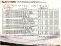 Research on analyzing the cost-volume-profit relationship in business decision making at animal feed processing enterprises in Vietnam - 25
 -
 Experiment 1: Study on the Effect of Potassium and Sulfur Fertilizer Dosage on Coffee and Tea Plants in the Business Stage on Red-Brown Basalt Soil in Lam Dong Province
 -
 Factors affecting business revenue and profit through satisfaction with the quality of transportation services of Quantium Vietnam Co., Ltd. - 8
 -
 Business Performance of Gia Music Training Center Revenue and Profit

Nguyen Minh Kieu 1 11/06/02
Fulbright Economics Teaching Program Financial Analysis Lecture 8
Lesson
Variable costs
3,000 | 10,500 | 4,500 | |
Operating profit (EBIT) | 5,000 | 4,000 | 10,750 |
Percentage change in EBIT | 400% | 100% | 330% |
(EBIT t – EBIT t -1 )/ EBIT t -1 |
1.2 Break-even analysis
Break-even analysis is a technique for analyzing the relationship between fixed costs, variable costs, profits, and sales volume. To illustrate the break-even analysis technique, let's take the following example: Suppose a bicycle manufacturing company has a unit selling price of $50, annual fixed costs of $100,000, and variable costs of $25/unit. We will analyze the relationship between total operating costs and total revenue. Figure 8.1 (page 3) illustrates the relationship between total revenue, total operating costs, and profits for each level of output and sales volume. It should be noted that here we are only interested in operating costs, so profits here are defined as operating profits before taxes. Thus, interest on debt and preferred dividends are not relevant when analyzing operating leverage. However, when analyzing financial leverage (later), we will consider this issue.
Figure 8.1 : Break-even analysis
Revenue and expenses ($1000)
Revenue
Total cost
Variable cost
Fixed cost
Production and consumption quantity
0
1000
2000
3000
4000
5000
6000
300
250
200
150
100
50
In Figure 8.1, the intersection point between the two lines of total revenue and cost is the break-even point because at this point revenue equals cost and, therefore, profit is 0. In Figure 8.1, the break-even point is the point where output is 4000. Mathematically, to find the break-even point we do the following:
Nguyen Minh Kieu 2
Fulbright Economics Teaching Program Financial Analysis Lecture 8
Lesson
Let EBIT = earnings before interest and taxes (operating profit) P = unit selling price
V = unit variable cost (P – V) = gross profit
Q = quantity produced and consumed F = fixed cost
Q BE = break-even quantity
At the break-even point, revenue equals costs and EBIT is 0. Therefore:
PQ BE = VQ BE + F (P – V)Q BE = F
Q BE = F/ (P – V) (8.1)
In the above example, if we apply formula (8.1), we will have break-even output Q BE = 100,000/ (50 – 25)
= 4,000 units. If the sales volume exceeds the break-even point (4,000 units), there will be a profit. Conversely, if the sales volume falls below the break-even point, the company will incur a loss.
The break-even point Q BE as determined above represents the break-even output. To find the break-even revenue, we multiply the break-even output by the unit selling price. In the above example, the break-even output Q BE = 4000 and the unit selling price P = 50$, so the break-even revenue will be 50 x 4000 = 200,000$.
1.3 Degree of operating leverage (DOL)
As analyzed in the previous section, we see that under the impact of operating leverage, a change in the number of sales results in a profit (or loss) increasing at a greater rate. To measure the impact of operating leverage, we use the degree of operating leverage (DOL). The degree of operating leverage (DOL) is defined as the percentage change in operating profit compared to the percentage change in output (or revenue). Therefore:
(8.2)
Percentage change in profit
operating profit Percentage change in output (or revenue)
Degree of operating leverage (DOL) at production level =
quantity Q (revenue S)
DOL
EBIT / EBIT
Q / Q
It should be noted that the degree of leverage may be different at different levels of output (or revenue). Therefore, when we talk about leverage, we should specify the leverage at a certain level of output Q or revenue S.
The above formula (8.2) is essential for defining and understanding the degree of operating leverage, but it is difficult to calculate in practice due to the difficulty of collecting EBIT data. To make the calculation of DOL easier, we make some changes. Knowing that gross profit equals revenue minus expenses, we have:
EBIT = PQ – (VQ + F) = PQ – VQ – F = Q(P – V) – F
Nguyen Minh Kieu 3
Fulbright Economics Teaching Program Financial Analysis Lecture 8
Lesson
Because the selling price P and fixed costs F are fixed, EBIT = Q(P – V). Thus:
EBIT EBIT
Q ( P V )
Q ( P V ) F
Substitute into formula (8.2), we get:
Q ( P V )
Q ( P V ) F
⎛ Q ( P V ) ⎞⎛ Q ⎞ Q ( P V )
DOL Q Q
⎜ ⎜ Q ( P V ) F ⎟ ⎟ ⎜ ⎜ Q ⎟ ⎟ Q ( P V ) F
DOL Q
⎝
Q
Q ( P V )
Q ( P V ) F
⎠⎝⎠
(8.3)
Dividing the numerator and denominator of (8.3) by (P – V), the formula (8.3) can be rewritten as:
Q ( P V )
DOL Q
( P V )
Q ( P V ) F
( P V )
Q
Q Q BE
(8.4)
Formulas (8.3) and (8.4) are used to calculate the degree of operating leverage in terms of output Q. These two formulas are only suitable for companies whose products are unique, such as cars or computers. For companies whose products are diverse and cannot be calculated in units, we use the degree of leverage based on revenue. The formula for calculating the degree of leverage based on revenue is as follows:
Nguyen Minh Kieu 4
Fulbright Economics Teaching Program Financial Analysis Lecture 8
Lesson
DOL S
S V
S V F
EBIT F
EBIT
where S is revenue and V is total variable costs.
Applying formula (8.4) to the example we have considered from the beginning of the lesson until now, we have:
So the degree of operating leverage at output level Q = 5000 is 5. What does this mean? It means
DOL 5000
DOL 6000
Q
Q Q BE
Q
Q Q BE
5000 5
5000 4000
6000 3
6000 4000
(8.5)
that is, from a sales volume of 5,000 units, for every percentage change in sales volume, operating profit changes by 5 percent. It should also be noted that when output increases from 5,000 to 6,000 units, the degree of operating leverage decreases from 5 to 3, meaning that from an output volume of 6,000 units, for every percentage change in sales volume, operating profit changes by 3 percent. Therefore, from the break-even point, the more output increases, the less leverage there is.
1.4 Relationship between operating leverage and break-even point
To see the relationship between operating leverage and the break-even point, we tabulate profits and operating leverage at different levels of output. Table 8.2 below shows us profits and operating leverage at different levels of output.
Table 8.2 : Profit and operating leverage at different levels of output
Production and consumption quantity
Operating profit (EBIT) | Degree of operating leverage (DOL) | |
(Q) | ||
0 | - 100,000 | 0.00 |
1000 | - 75,000 | - 0.33 |
2000 | - 50,000 | - 1.00 |
3000 | - 25,000 | - 3.00 |
Q BE = 4000 | 0 | Unknown |
5000 | 25,000 | 5.00 |
6000 | 50,000 | 3.00 |
7000 | 75,000 | 2.33 |
8000 | 100,000 | 2.00 |
Table 8.2 shows that the further the volume moves from the break-even point, the greater the operating profit or loss, and conversely the smaller the degree of operating leverage (DOL). The relationship between volume and operating profit is linear as shown in Figure 8.1. Figure 8.2 below illustrates the relationship between volume and operating leverage.
Nguyen Minh Kieu 5
Fulbright Economics Teaching Program Financial Analysis Lecture 8
Lesson
Figure 8.2 : Relationship between sales volume and operating leverage
Operating leverage
5
3
2
1
0 2000 3000
- 1
- 3
4000 5000 6000
8000
Production and consumption quantity
Figure 8.2 gives us some observations as follows:
The degree of operating leverage approaches infinity as the quantity produced and sold approaches the break-even point.
As production and consumption volumes move further beyond the break-even point, the degree of leverage approaches 1.
1.5 Relationship between operating leverage and business risk
Business risk is the risk that operating profits will decline due to fluctuations in the operations of a business. It should be noted that operating leverage is only one component of business risk. Other elements of business risk are the variability or volatility of revenues and costs of production. These are the two main elements of business risk, and operating leverage amplifies the impact of these factors on the operating profits of a business. However, operating leverage itself is not the source of risk, because high leverage is meaningless if revenues and fixed cost structures are fixed. Therefore, it would be wrong to equate operating leverage with business risk, because the root is variability in revenues and costs of production, but operating leverage has the effect of amplifying the variability of profits and, therefore, business risk.
From this perspective, operating leverage can be viewed as a form of potential risk that only becomes an operating risk when there are fluctuations in revenue and production costs.
1.6 The significance of operating leverage for financial management
After studying operating leverage, let us ask the question: How is understanding a company's operating leverage useful to a CFO? As a CFO, you need to know in advance how changes in revenue will affect operating profit. Operating leverage is a tool that helps you answer this question. Sometimes knowing the operating leverage in advance can help a company decide its revenue and cost policies more easily. But in general, companies do not like to operate under conditions of high operating leverage because in such a situation, a change in operating leverage is all it takes.
Nguyen Minh Kieu 6