entangled state. As β increases, the second peak of
E 20 split into two vertices and they
E
Maybe you are interested!
-

 Factors affecting budget estimates at State Reserve Department units in the Southeast region - 13
 -
 Determining the price of residential land for compensation when the State recovers land according to current Vietnamese law - 2
 -
 Directions for Improving State Management of Tourism Activities in Dak Nong Province
 -
 State management of compensation, support and resettlement when the State acquires land in Buon Ho town, Dak Lak province - 12
 -
 The impact of state ownership and bank loans on investment decisions of companies in Vietnam - 18
3
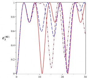
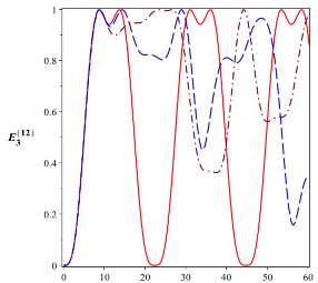
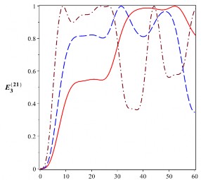
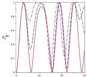
reaches approximately unity and the period of the entanglement entropies changes. Therefore, the presence of β changes the values and positions of the peaks of the entanglement entropy.
entanglement. Furthermore, in the same time interval, the entanglement entropies have more maxima than the results of [23].
02
E
3
and 12
t [10 -6 s ] t [10 -6 s ]
t [10 -6 s ] t [10 -6 s ]
1
2
2
1
2
0
Figure 2.19: Evolution of entanglement entropy (in ebit units) of the cut state for the
0
2
ab
initial state is


( E 02 ),


 ( E 12 ),


( E 21 ) and


( E 20 ) with
3
3
3
3
ab
ab
ab
4 10 4 rad/s. The solid line is for 0 , the dashed line is for
2 10 4 rad/s and the dotted line is for 4 10 4 rad/s
ab
ab
Figures 2.20 to 2.25 show the probabilities for the system to exist in the states
Bell's Slice
aba
 2 1
2 1

 and
and 2
2
mn i 3

B
b
 0 .
0 .
( i =1,2,3,...,6) correspond to the initial states 0

 2
2
, 1
1
 2 ,
2 ,
t [10 -6 s ] t [10 -6 s ]
t [10 -6 s ] t [10 -6 s ]
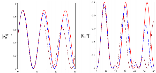
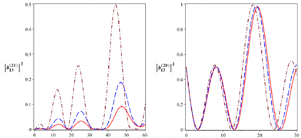
Figure 2.20: Probability for the system to exist in Bell-type states
02


B
0
2
,
ab
13
( b 02 2 ),
12


B
13


13
13
B
( b 12 2 ),
21 13
( b 21 2 ) and
20 13
( b 20 
 2 ) correspond to the initial states


13
B
13
ab
2 1
2 0
ab
and
ab
 1
1
 2
2 ,
,


with 4 10 4 rad/s. The solid line is for
0 , line
dash is for
2 10 4 rad/s and the dotted line is for
4 10 4 rad/s
t [10 -6 s ] t [10 -6 s ]
t [10 -6 s ] t [10 -6 s ]
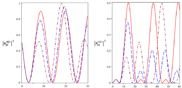
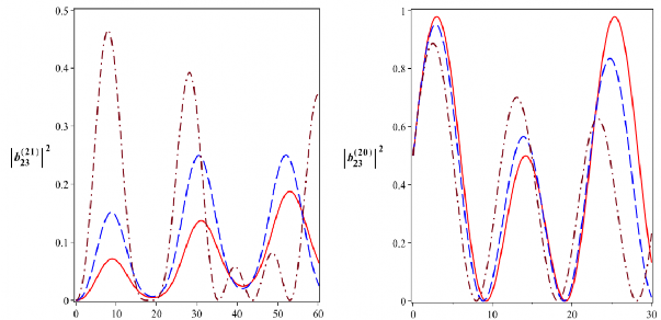
Figure 2.21: Probability for the system to exist in Bell-type states
02


B
0
2
,
ab
23
( b 02 2 ),
12


B
23


23
23
B
( b 12 2 ),
21 23
( b 21 2 ) and
20 23
( b 20 
 2 ) correspond to the initial states


23
B
23
ab
2 1
2 0
ab
and
ab
 1
1
 2
2 ,
,


with 4 10 4 rad/s. The solid line is for
0 , line
dash is for
2 10 4 rad/s and the dotted line is for
4 10 4 rad/s
t [10 -6 s ] t [10 -6 s ]
t [10 -6 s ] t [10 -6 s ]
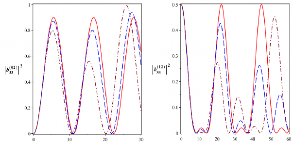
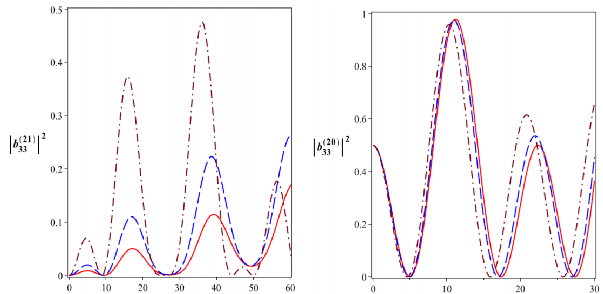
Figure 2.22: Probability for the system to exist in Bell-type states
02


B
0
2
,
ab
33
( b 02 2 ),
12


B
33


33
33
B
( b 12 2 ),
21 33
( b 21 2 ) and
20 33
( b 20 
 2 ) correspond to the initial states


33
B
33
ab
2 1
2 0
ab
and
ab
 1
1
 2
2 ,
,


with 4 10 4 rad/s. The solid line is for
0 , line
dash is for
2 10 4 rad/s and the dotted line is for
4 10 4 rad/s
t [10 -6 s ] t [10 -6 s ]
t [10 -6 s ] t [10 -6 s ]
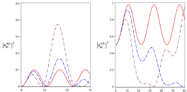
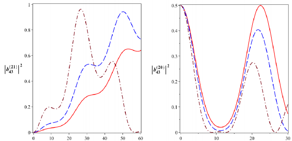
Figure 2.23: Probability for the system to exist in Bell-type states
02


B
0
2
,
ab
43
( b 02 2 ),
12


B
43


43
43
B
( b 12 2 ),
21 43
( b 21 2 ) and
20 43
( b 20 
 2 ) correspond to the initial states


43
B
43
ab
2 1
2 0
ab
and
ab
 1
1
 2
2 ,
,


with 4 10 4 rad/s. The solid line is for
0 , line
dash is for
2 10 4 rad/s and the dotted line is for
4 10 4 rad/s
t [10 -6 s ] t [10 -6 s ]
t [10 -6 s ] t [10 -6 s ]
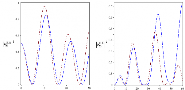
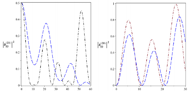
Figure 2.24: Probability for the system to exist in Bell-type states
02


B
53
0
2
,
ab
53
( b 02 2 ),
12


B
53


53
53
B
( b 12 2 ),
21 53
( b 21 2 ) and
20 53
( b 20 
 2 ) correspond to the initial states


53
B
ab
2 1
2 0
ab
and
ab
 1
1
 2
2 ,
,


with
4 10 4 rad/s. The dashed line is for
2 10 4 rad/s and the dotted line is for 4 10 4 rad/s
t [10 -6 s ] t [10 -6 s ]
t [10 -6 s ] t [10 -6 s ]
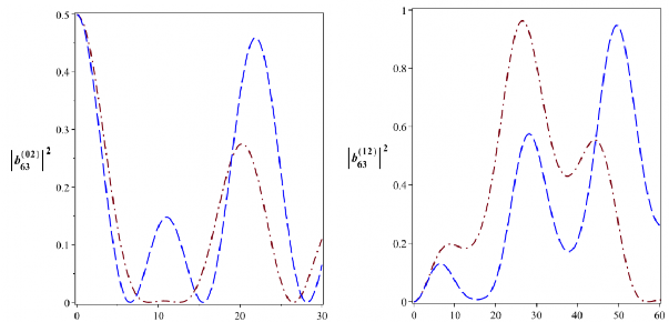
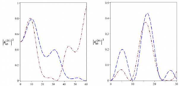
Figure 2.25: Probability for the system to exist in Bell-type states
02


B
63
0
2
,
ab
63
( b 02 2 ),
12


B
63


63
63
B
( b 12 2 ),
21 63
( b 21 2 ) and
20 63
( b 20 
 2 ) correspond to the initial states


63
B
ab
2 1
2 0
ab
and
ab
 1
1
 2
2 ,
,


with
4 10 4 rad/s. The dashed line is for
2 10 4 rad/s and the dotted line is for 4 10 4 rad/s
When β = 0, we obtain the results of the case of a single-mode injected nonlinear coupling presented in section 2.2.1. In particular, for the initial state


a
b
is 2 0 , the result obtained for the case β = 0 also coincides with the probability that the system
exist in Bell-type states pumped by one mode by the external field discussed in [23]. When β = α, we also obtain the probabilities for the system to exist in Bell-type states pumped by two external fields of the same strength [109].
and
From Figures 2.20 to 2.25, we see that the maximum entanglement states
can be generated for all four initial states.
 0
0
 2
2 ,
,
 1
1
 2
2 ,
,


with


ab
ab
2 1
2 0
B
B
B
ab
ab
and
and
and
different values of the parameter β . Specifically, the maximal entanglement states


B
02
B
13
and
20 13
(Figure 2.20),
02


B
23
and
20 23
(Figure 2.21),
02


B
33
and
20 33
(Image
2.22),
12


B
43
21 43
(Figure 2.23),
02


B
53
20 53
(Figure 2.24),
12


B
63
21 63


B
B
(Figure 2.25) can be created, otherwise the states
12


B
,
13
21 13
12


B
,
23


B
B
,
21 23
12


B
,
33
21 33
02


B
,
43
20 43
12


B
,
53
21 53
02


B
63
20 63
cannot create


B
B
B
B
B
B
,
,
,
and
and
produce maximally entangled states. Thus, in the same Bell-type state for four different initial conditions, two initial conditions can produce Bell-type states, while the remaining two initial conditions cannot produce Bell-type states.
Bell-type state in pairs
20


B
i 3
02


B
and
i 3
or
12
i 3
21
i 3
. When β


B
B
B
increasing, in a Bell-type state for four different initial conditions, for two initial conditions the probability values of the states increase, while for the remaining two initial conditions the probability values of the states decrease. The states


B
20 13
(Figure 2.20),
02
23
(Figure 2.21),
02
33
(Figure 2.22),
21 43
(Figure 2.23),


B
and
02
53
20 53
(Figure 2.24),
12


B
63
21 63
(Figure 2.25) is approximately equal to the unit


B
B
and
that is, Bell-type states are generated with high precision, while the remaining states hardly generate Bell-type states. More