Complexity Assessment and Algorithm Implementation

- The function buildJPlan x (a u(x), b v(x) ) combines plans a u(x) and b v(x) into a plan in which the results of T r,p and T i-r,q at station x are implicitly connected at this station, that is buildJPlan x (a u(x), b v(x) ) = IJ x (a u(x), b v(x) ). The notation c w(x) is the plan generated by the above function. By executing this plan, the results of T i,j are explicitly calculated at station x.

- The function buildTPlan x,t (c w(x) ) extends the plan into another plan in which the results of T i,j at station x are transmitted to station t, buildTPlan xt (c w(x) ) =TR x,t (c w(x) ). Executing this plan will obtain the results of T i,j at station t.

Since the results of T r,p and T i-r,q must be at the same station to be implicitly joined, the cost of the plan generated by buildJPlan x (a u(x), b v(x) ) is the sum of the costs of fetching the results of the queries T r,p and T i-r,q at station x and the cost of the implicit join at this station. Similarly, the cost of the plan generated by buildTPlan x,t (c w(x) ) is the sum of the costs of the results

explicitly compute the query at station x and the cost of transmitting the result of query T i,j from station x to station t. Therefore, we have:

Cost(buildJPlan x (a u(x), b v(x) ))=Cost(a u(x) )+Cost(b v(x) )+join x (T r,p ,T i-r,q ) (3.6) Cost(buildTPlan x,t (c w(x) )) = Cost(c w(x) )) + trans x,t (T ij ) (3.7) where join x (T r,p ,T i-r,q ) is the cost of the implicit join between the results T r,p and

T i-r,q at station x and trans x, t (T i,j ) is the cost of transmitting the result of T i,j from station x to station t.

To select an optimized plan among the plans generated by buildJPlan and buildTPlan respectively, the optimization principle is used: If the plans differ only in their subplans, the plan with the optimal subplan is the optimal plan. This principle can be expressed formally as follows:

Cost(a l(x) )<=( ∀ u) Cost(a u(x) ) and Cost(b l(x) )<=( ∀ v) Cost(b v(x) )

=>Cost(buildJPlan x (a l(x), b l(x) ))<=( ∀ u,v) Cost(buildJPlan x (a u(x), b v(x) )) (3.8) Cost (c l(x) ))<=( ∀ w) Cost(c w(x) ))

=> Cost(buildTPlan x,t (c l(x) ))<=( ∀ w) Cost(buildTPlan x,t(c w(x) )) (3.9)

Where the sub-plans a l(x), b l(x) and c l(x) are the lowest cost plans among the plans a u(x), b v(x) and c w(x) respectively .

Theorem 3.1: The cost model for the implicit connection plan and the transmission plan satisfies the optimization principle.

Proof: To prove the theorem, we prove expressions (3.8) and (3.9). The proof for formula (3.8) is as follows, where steps 1 and 3 follow the definition of cost of buildJPlan and step 2 is due to the assumption that Cost(a l(x) )<=Cost(a u(x) )

and Cost(b l(x) )<=Cost(b v(x) ) for arbitrary values ​​of u and v.

Cost(buildJPlan x (a l(x), b l(x) )) = Cost(a l(x) ) + Cost(b l(x) ) + join x (T r,p , T i-r,q )

<= Cost(a u(x) ) + Cost(b v(x) ) + join x (T r,p , T i-r,q )

<= Cost(buildJPlan x (a u(x), b v(x) ))

The proof of formula (3.9) is as follows, where step 1 and step

3 according to the cost definition of buildTPlan and step 2 is due to the assumption that Cost(c l(x) )<=Cost(c w(x) ) for arbitrary w values.

Cost(buildTPlan x,t (c l(x) )) = Cost(c l(x) )) + trans x,t (T i,j )

<= Cost(c w(x) )) + trans x,t (T i,j )

<= Cost(buildTPlan x,t (c w(x) ))

3.4.5. PathExpOpt optimization algorithm

The algorithm consists of the following three steps:

 The first step is initialization

 The next step is to find the optimal solution for the induced subtrees, from trees with one vertex to trees with n vertices.

 The final step executes the path expression according to the found optimal plan.

a. Initialization

 In the initialization section, reduce the classes (or class fragments) by projections on the attributes that need to be left, these attributes belong to one of the following three types:

o OIDs of classes

o Complex attributes used for concatenation

o Attributes to select after query

 Generate sympathetic plantlets and calculate the size of the sympathetic plantlets.

b. Find the optimal solution

- Step 1: Initialize the cost of single-vertex trees, the cost of single-vertex trees at each station is the cost of transmitting vertices to this station.

- Step 2: Build optimal solutions for trees from 2 vertices.

o Step 2.2: Find the optimal implementation plan for T i, j through the transmission operations. The cost of T i, j at station t will be recalculated if this cost is greater than the total cost of T i, j at station x and the transmission cost of T i, j from station x to station t. Save the optimal implementation plan.

Algorithm 3.5 PathExpOpt Input:

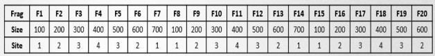
- G =(V, E); V={F 1 , F 2 ,…, Fn};

- fragSize: Array that stores the size of the fragments

- fragSite: The array of stations where the fragments are located

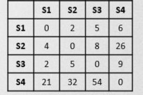
- transCost: Array to store costs between stations

- T: The induced subtrees of the original query tree

- treeSize: Array of tree sizes, calculated when the tree is generated.

- k: Query generating station

Output: Optimal execution plan for the query tree (result) Algorithm steps:

//Step 1: Initialize the cost of 1-vertex subtrees for (u=1; u<=n; u++) //n is the number of pieces

begin

x = fragSite u ;

for (t = 1; t<=s; t++) //s is the number of stations Cost_Trans t (T 1,u )= fragSize u * transCost x,t ;

end; {for u}

//Step 2: Build optimal solutions for trees from 2 vertices for (i=2; i<=n; i++)

//Step 2.1: Find the optimal solution to implement T i,j through the joins for (j=1; ji ; j++) //m i is the number of induced seedlings with i vertices

for (t = 1; t<=s; t++)

JoinPlan t (T i,j )= Find_JoinPlan(T i,j ); end; end; {for t}

end; {for j}

//Step 2.2: Find the optimal solution to implement T i,j through propagation

for (t = 1; t<=s; t++) for (j=1; ji ; j++)

TransPlan t (T i,j )= Find_TransPlan t (T i,j ); end; end; {for j}

end; {for t} end; {for i}

result = TransPlan k (T n,1 ); //k is the station that generates the query

end; {Algorithm 3.5}

Algorithm 3.6 Find_JoinPlan(T i,j )

//Find the optimal solution to implement T i,j through the connections Input :

- G =(V, E); V={F 1 , F 2 ,…, Fn};

- transCost: Array to store costs between stations

- T: The induced subtrees of the original query tree

- treeSize: Array of sizes of the subtrees, calculated when the tree is generated

Output: JoinPlan t (T i,j ). Steps of the algorithm:

//Find the smallest cost of the induced subtree T i,j at the stations Cost_Join t (T i,j )=∞ ;

// Browse tree splitting methods

for (each (T r,p and T i-r,q ) that T i,j = T r, p ᴜ T i-r,q ) begin

//calculate the cost of joining T r,p and T i-r,q according to the Bloom filter Cost_Temp = cost_BloomJoin t (join(T r,p ,T i-r,q );

if (Cost_Join t (T i,j )>cost_Temp) begin

//save small cost plan Cost_Join t (T i,j )= cost_Temp; save JoinPlan t (T i,j );

end; {if}

end; {for each}

end; {Algorithm 3.6}

Algorithm 3.7 Find_TransPlan(T i,j ).

//Find the optimal solution to implement T i,j through the following operations Input:

- G =(V, E); V={F 1 , F 2 ,…, Fn};

- transCost: Array to store costs between stations

- T: The induced subtrees of the original query tree

- treeSize: Array of sizes of the subtrees, calculated when the tree is generated

Output: TransPlan t (T i,j ) Steps of the algorithm:

//Consider if there is a solution where the total cost of joining on a station is

//that plus the transmission cost to this station is smaller then replace Cost_Trans t (T i,j )= ∞ ;

for (x = 1; x<=s; x++)

begin

Cost_Temp = Cost_Join x (T i,j )+ treeSize(T i,j )* transCost x,t; if (Cost_Trans t (T i,j )>cost_Temp)

begin

//replace the connection at t with a connection at x and then pass it to t Cost_Temp t (T i,j )= cost_Temp;

save TransPlan t (T i,j ); end; end; {if}

end; {for x}

end; {Algorithm 3.7}

c. Execute the query according to the optimal plan

By going backwards from the tree Tn ,1 will find the optimal plan and execute the query according to this optimal plan. During the execution, Bloom filter is used to transfer data.

3.4.6. Complexity assessment and algorithm implementation

The complexity of the algorithm depends on the number of layers, the number of stations and the number of generated subtrees. In the best case, the query graph is a string graph (corresponding to a string query), then the number of generated subtrees with i vertices is n-i+1, then the number of join plans and transfer plans is:

𝑛 𝑛−𝑖+1 𝑠

𝑖−1

𝑠 𝑛−𝑖+1 𝑠

(𝑛 − 1)𝑛(𝑛 + 1) (𝑛 − 1)𝑛

∑( ∑ ∑ ∑ 𝑟 + ∑ ∑ ∑ 𝑥) = 𝑠 + 𝑠 2

(3.10)

𝑖=2

𝑗=1

𝑡=1 𝑟=1

𝑡=1

𝑗=1

6 2

𝑥=1

𝑖−1

Thus, the best case complexity of the algorithm is O(sn 3 ). In the worst case, the query graph is a star graph (corresponding to a star query), the number of induced subtrees is 𝐶 𝑛−1 , the complexity of the algorithm in this case is

O(s2 n-1 ).

𝑛

𝑛−1

𝐶

𝑖−1 𝑠

𝑖−1

𝑛−1

𝐶

𝑠 𝑖−1 𝑠

∑( ∑ ∑ ∑ 𝑟 + ∑ ∑ ∑ 𝑥) = 𝑠(𝑛 − 1)2 𝑛−2 + 𝑠 2 (2 𝑛−1 − 1) (3.11)

𝑖=2

𝑗=1

𝑡=1 𝑟=1

𝑡=1

𝑗=1 𝑥=1

In the case of a query graph with many induced subgraphs, a heuristic can be used for the algorithm by considering only the ways to split T i,j into trees T 1,p and T i-1,q . Experiments show that the execution time of the algorithm for a 20-vertex star graph from 15 minutes when using the above heuristic is only less than 1 minute, the resulting solution is a near-optimal solution with a cost not much different from the optimal solution.

The algorithm was implemented in Java and tested with path expression queries involving a class number of 20.

3.4.7. Experimental results

An example of experimental data and the generated results is shown in Figure 3.6. The experimental data consists of a set of 20 fragments belonging to classes with predetermined sizes and stations, the connection graph is a star-shaped graph with many nodes, the connection network consists of 4 stations with a predetermined cost of transmitting each unit of data between 2 stations.

T[11,2492]: 4,7,5,6,10,11,16,17,18,19,20

1: T[1,4] + T[10,2312] = [12400, 17000, 25400, 4600]

2: T[1,5] + T[10,1850] = [6800, 8000, 5600, 8500]

3: T[1,16] + T[10,1388] = [6600, 5500, 7200, 9800]

4: T[1,17] + T[10,1387] = [6400, 7000, 5600, 7300]

5: T[1,18] + T[10,1386] = [14200, 18300, 27200, 6400]

6: T[1,19] + T[10,1385] = [6800, 8000, 5600, 9100]

7: T[1,20] + T[10,1384] = [8200, 5500, 10400, 20200]

8: T[3,5] + T[8,1346] = [7100, 6900, 7900, 5600]

9: T[4,6] + T[7,950] = [7600, 6900, 7800, 6100]

10: T[5,10] + T[6,515] = [8200, 8100, 7800, 6700]

- JOIN: [6400, 5500, 5600, 4600]

- J_PLAN: [[1,17]+[10,1387], [1,16]+[10,1388],

[1,5]+[10,1850], [1,4]+[10,2312]]

- TRANS: [5800, 5500, 5600, 4600]

- T_PLAN: [3, 0, 0, 0]

JOIN_2(F2,JOIN_2(F9,JOIN_2(F13,JOIN_2(F16,JOIN_2(F20,TRANS_1->2(JOIN_1(F8,JOIN_1(F14, JOIN_1(F15,TRANS_3->1(JOIN_3(F3,JOIN_3(TRANS_1->3(F1),JOIN_3(F5,JOIN_3(F17,JOIN_3(F19, TRANS_1->3(JOIN_1(TRANS_3->1(F12),TRANS_4->1(JOIN_4(F4,JOIN_4(F18,JOIN_4(F11,

TRANS_1->4(JOIN_1(F7,TRANS_2->1(JOIN_2(F6,TRANS_3->2(F10))))))))))))))))))))))))))

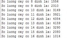
Figure 3.6: Illustration of test results