A Modified Research Model on the Impact of Training Service Quality on Student Satisfaction at Saigonact School

*Determine the importance of variables in the model:

The components in the model include: teaching staff, office staff work in the school, training programs, school reputation, student access to services, and understanding of students. These are the components that have important impacts on student satisfaction. The order of importance of each component depends on the absolute value of the standardized regression coefficient. The component with the larger absolute value has a greater impact on satisfaction. Therefore, in this model we see that student satisfaction is most influenced by the composition of the teaching staff (beta = 0.340), the second most important is the training program component (beta = 0.302), the third component is the work of office staff (beta = 0.182), the fourth is the reputation of the school (beta = 0.171), the fifth is the component of caring and understanding students (beta = 0.149) and the sixth is the component of student access to services (beta = 0.090).

The results of the regression coefficient analysis show that the model does not violate the multicollinearity phenomenon because the variance inflation factor (VIF) of the independent variables is less than 2. The results of the regression coefficient analysis show that the Sig. value of all independent variables is less than 0.05. Therefore, it can be said that all independent variables are significant in the model and have a positive impact on student satisfaction (because the regression coefficients are all positive).

*Building a linear regression equation

The regression equation has the following form:

HL = B 0 + B 1 NV i + B 1 GV i + B 1 DT i + B 1 TC i + B 1 CTDT i + B 1 QT i + e i

Based on coefficient B, we have the following regression equation:

HL = 0.221 + 0.149NV i + 0.283GV i + 0.143DT i + 0.075TC i + 0.251CTDT i + 0.126QT i + e i

4.4.5 Testing research hypotheses

This model explains 84% of the variation in the satisfaction variable (HL) due to the independent variables in the model, the remaining 16% of the variation is explained by other variables outside the model. The model shows that the independent variables all have a positive (directed) effect on the level of student satisfaction with a confidence level of 95%.

Table 4.18. Summary results of hypothesis testing

Hypothesis	Significance level (Sig.)	Results
H1	Teaching staff positively affects student satisfaction	0.000	Accept
H2	Office worker job positively affects student satisfaction	0.000	Accept
H3	Training program positively affects student satisfaction	0.000	Accept
H4	School reputation positively affects student satisfaction.	0.004	Accept
H5	Student service accessibility positively affects student satisfaction.	0.000	Accept
H6	Empathic concern for students positively affects student satisfaction	0.000	Accept

Maybe you are interested!

*Research model calibration

Student satisfaction

Office worker work 0.182

Personal characteristics

Teaching staff 0.340

School reputation 0.171

Student access to services 0.090

Training program 0.302

Understanding and care 0.149

Figure 4.4. Calibrated research model on the impact of training service quality on student satisfaction at SaigonACT school

In the model, the author will adjust one component in the components that make up the quality of training services, which is the training program component. Specifically, the variable CTDT4 (The school's training program creates more interest in learning for students) in the school's training program component will be removed.

4.4.6 By finding violations of necessary assumptions in linear regression

*Assuming linear relationship

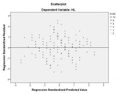
Figure 4.5. Linear relationship test results (Source: author's calculation)

From the above graph, it is shown that the linearity assumption is satisfied because their residuals are randomly scattered in a region around the line passing through the zero-ordinate axis and do not form any shape. This shows that the test results of the linearity relationship assumptions are appropriate, accepting the calibrated research model.

*The variance of the residuals is constant

Hypothesis H 0 : The correlation coefficient of the population is 0

Table 4.19. Results of the test for constant variance of residuals

Correlations

			HL	ABSCUARE
Spearman rho method	Satisfied	Correlation coefficient	1,000	,407
		Sig. (2-tailed)		0.000
		Overall - N		287
	ABSCUARE	Correlation coefficient	,407	1,000
		Sig. (2-tailed)	0.000
		Overall - N	287	287

(Source: author's calculation)

The test results demonstrate that there is not enough evidence to reject the null hypothesis H0 , which means that the variance of the error is constant.

*Normal distribution of residuals

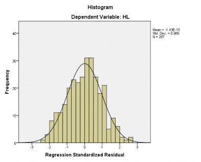
Figure 4.6. Normal distribution results of residuals

(Source: author's calculation)

From the histogram it can be seen that there is a normal distribution curve superimposed on the histogram, it would be unreasonable to expect that the observed residuals have a completely normal distribution, as there is always a sampling bias, the results from the histogram show that the residuals are approximately normal since the mean value Mean = 0 and the standard deviation Std.Dev = 0.989 or it can be said to be close to 1, from which it can be concluded that the normal distribution hypothesis is not violated.

*Independence of residuals

Hypothesis H 0 : The overall correlation coefficient of the residuals is 0

Table 4.20. Results of testing the independence of residuals

Model

R	R2	R2 adjustment	Estimated standard deviation	Durbin Watson Statistics
1	0.917 (a)	0.842	0.843	0.24308703	1,909

(Source: author's calculation)

From the Durbin Watson result it is very low (d = 1.909) meaning that the residuals close together are positively correlated.

*Multicollinearity phenomenon

Hypothesis H 0 : independent variables are not correlated with each other

From the test results in Table 4.17, it can be seen that the model does not violate the multicollinearity phenomenon because the variance inflation factor (VIF) of the independent variables is less than 2, so there is enough basis to reject the hypothesis H0 , which means that the independent variables are closely correlated with each other.

4.5 Test the difference in the level of assessment of training service quality components affecting student satisfaction according to personal characteristics.

In this study, the author uses Independent Samples T-test and One-Way ANOVA analysis to investigate the level of satisfaction with the quality of training services of students by faculty, gender and course. The research problem here is whether the level of importance of student satisfaction is different between students of faculties, genders and academic years. We hypothesize:

H 0 : The level of student satisfaction with the quality of training services (according to different faculties, different genders, different academic years) is the same. This means that there is no difference in the level of student satisfaction with the quality of training services. In this analysis, the coefficient of interest is the sig coefficient. If the sig coefficient. ≤ 0.05 (with a significance level of 95%), then reject the hypothesis H 0 , meaning there is a difference in the assessment results of the subjects on the importance of the factors. If Sig > 0.05, then accept the hypothesis H 0.

4.5.1 Testing for gender differences

Table 4.21. Results of testing for gender differences

Independent Samples Test

Levene's Homogeneity of Variance Test				Homogeneity of means test (t-test)
Levene's Homogeneity of Variance Test				(a) Homogenous variance				(b) Heterogeneous variance
		F	Sig.	T	Df	Sig. (2-tailed)	Mean deviation	Standard deviation	95% confidence interval
		F	Sig.	T	Df	Sig. (2-tailed)	Mean deviation	Standard deviation	Lower	Higher
NV	A	3,526	,061	,100	285	,920	,00975610	,09707802	-,18132476	,20083696
NV	B			,094	130,883	,925	,00975610	,10378641	-,19555988	,21507208
GV	A	,011	,915	,667	285	,505	,06341463	,09506861	-,12371107	,25054033
GV	B			,675	152,922	,501	,06341463	,09399509	-,12228191	,24911118
DT	A	,402	,526	-,289	285	,773	-,02731707	,09460107	-,21352250	,15888836
DT	B			-,300	162,486	,764	-,02731707	,09098886	-,20699017	,15235603
TC	A	,126	,723	,474	285	,636	,04512195	,09519969	-,14226176	,23250566
TC	B			,479	152,924	,632	,04512195	,09412395	-,14082915	,23107305
CTDT	A	,130	,718	,308	285	,758	,02926829	,09502753	-,15777655	,21631314
CTDT	B			,306	147,155	,760	,02926829	,09568135	-,15981874	,21835532
QT	A	,089	,766	1,254	285	,211	,11707317	,09335045	-,06667063	,30081697
QT	B			1,259	150,386	,210	,11707317	,09302335	-,06672832	,30087467
HL	A	1,058	,304	,205	285	,837	,01626016	,07914119	-,13951524	,17203556
HL	B			,212	158,987	,833	,01626016	,07686455	-,13554712	,16806744

(Source: author's calculation)

From the T-test results, it shows that all Sig. values in the Levene test of all components are greater than 0.05, so we use the t-test results in the Equal variances assumed section. Seeing that all Sig. values are greater than 0.05, it can be said that there is no difference in the evaluation of the components of training service quality affecting satisfaction by gender.

Table 4.22. Mean values by gender

Report – Report

Sex		NV	GV	DT	TC	CTDT	QT	HL
Male	Medium	3,543	3,496	3,551	3,315	3,553	3,561	3,813
Male	N	291	287	291	272	291	292	313
Female	Medium	3,533	3,433	3,579	3,270	3,524	3,444	3,797
Female	N	724	704	734	670	722	706	778
Total	Medium	3,536	3,451	3,571	3,283	3,532	3,477	3,801
Total	N	1015	990	1025	942	1014	998	1091

(Source: author's calculation)

Table 4.22. above shows that there is not much difference in the assessment of training service quality between men and women.

4.5.2 Testing for differences by subject area

Table 4.23. Testing results by major

Test for homogeneity of group variances

(Test of Homogeneity of Variances)

	Levene Statistics	df1	df2	Sig.
NV	,803	3	283	,493
GV	,534	3	283	,659
DT	,881	3	283	,451
TC	,558	3	283	,643
CTDT	,106	3	283	,956
QT	,625	3	283	,599
HL	,534	3	283	,659

(Source: author's calculation)

Through table 4.23. we see that with the significance level Sig. of the independent variables all greater than 0.05, it can be said that the variance of the 4 groups of majors in assessing the importance of the components is not different and is not statistically significant. Therefore, the author did not conduct ANOVA analysis to learn more about this personal characteristic.

4.5.3 Testing the difference in the number of years of study of students Table 4.24. Testing results according to the number of years of study

Test for homogeneity of group variances

(Test of Homogeneity of Variances)

	Levene Statistics	df1	df2	Sig.
NV	,288	2	284	,750
GV	,054	2	284	,947
DT	,865	2	284	,422
TC	3,150	2	284	,044
CTDT	,117	2	284	,889
QT	1,389	2	284	,251
HL	2,913	2	284	,056

(Source: author's calculation)

Through table 4.24. we see that the significance level Sig. of the independent variables is almost all greater than 0.05, it can be said that the variance of the 3 groups of years of study (K7, K8, K9) of students in assessing the importance of the components is not different and not statistically significant. Only the component of student service access is the opposite. Therefore, the author included this factor in ANOVA analysis to study specifically.

Table 4.25. Results of variance test according to number of years studied

Analysis of variance – ANOVA