A General Model of Tourist Destination Perception and Choice

perceptions are not available and the group is not adapted. Different destinations will appeal to different tourists based on how well the marketing meets their individual needs. Customers will consider purchasing these brands based on how likely they believe the brand will meet their needs.

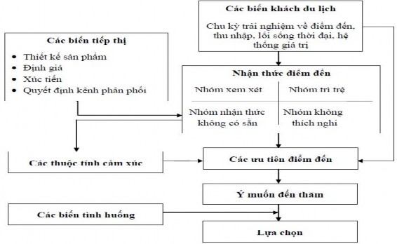
Figure 2.3: General model of tourism destination perception and choice

Source: Woodside and Lysonski (1989, p. 9).

However, in developing a model of the destination choice process, Pearce (2005) pointed out the challenges for destination choice models: (1) travel is not just a single destination but a multi-destination trip; (2) choice models often represent an individual's choice process, but the concept of shared, focal or social decision making is not fully developed in the existing literature; (3) different types of decision making processes such as decisions for countries, entire regions and within a region, or for day trips, short holidays and longer vacations. It is also important to note that destination choice intentions and actual destination choice are not the same concept. According to the theory of planned behavior (TPB) as well as in practice, intended behavior is often found to have a major impact on actual behavior but

It cannot be denied that what people ultimately care about is the actual behavior. Therefore, for the purpose of this study, the author uses the general tourism model of Woodside and Lysonski (1989) to focus on the study of tourists' actual destination choice.

2.6.2. Approaches

Mansfeld (1992) argues that there are two theoretical approaches from previous studies to study tourists' destination choice decision making:

(1) Approach based on neoclassical traditional demand theory and (2) Approach based on

on random utility theory.

The first approach from the utility (value) perspective is based on the neo-classical traditional demand theory, the concept of “economic-rational man” means that tourists have a spatial arrangement reflecting their need to optimize their utility within the constraints of time and money (Girt, 1976; Halperin et al., 1984; Nicolau and Más, 2006). In this theory, the three factors of income, price (relative), and taste are considered the foundation of tourism demand analysis. Tourists will choose the consumption bundle that is the point of tangency between the budget line and the highest indifference curves to maximize their utility.

This theory suggests that when tourists make decisions, they will compare the expected benefits of each alternative in a set of destinations defined by their attributes. Although utility is an unobservable quantity, one can observe the actual choices of tourists and therefore the ranking of the benefits of each alternative can be derived from the observation. However, this approach has been criticized as unrealistic (Rugg, 1973; Mansfeld, 1992; Papatheodorou, 2001). Since a potential tourist can travel to one of many destinations by many different modes, the list of destinations that will be substituted into the traditional utility functions is very large (Rugg, 1973). In addition, tourists' destination choices, with many different types of options, involve a degree of uncertainty (Mansfeld, 1992). On the other hand, this approach ignores the possibility of the emergence of new destinations and the destruction of existing ones.

of old destinations and does not take into account some factors that differentiate the tourism product (Papatheodorou, 2001). These limitations explain why the theory does not take into account the importance of product differentiation and excludes the effects of tourists' attitudes towards the services and attributes of the destination.

To address the problems raised by traditional demand theory in the tourism field, Lancaster’s attribute approach is used in studies to understand tourism demand and tourist behavior. Based on this theory, demand for a product is derived from the benefits received by the intrinsic attributes of the product rather than by the product itself (Lancaster, 1966). Consumers will choose the combination of products that provides the optimal basket of attributes embodied in each product. This theory assumes that product attributes are either additive or combinable. Several scholars such as Rugg (1973), Morley (1994), Lise and Tol (2000), Papatheodorou (2001), Seddighi and Theocharous (2002), Zhang et al. (2004), Aguiló et al. (2005), Naude and Saayman (2005), Lyons et al. (2009), Kuawiriyapan et al. (2010), Li et al. (2011), Liu and Ko (2011) have applied the attribute approach in tourism. In these studies, the service characteristics of the destination are the decisive criteria for the construction of tourists' attitudes and perceptions towards alternative destinations. However, Lancaster's theory also has its own drawbacks. According to Hendler (1975), the attribute demand theory depends on the ability to distinguish between objective and subjective choices. The theory is said to be relevant only under certain assumptions, where there is no criterion for assessing consumer efficiency, unless the goods are known to be mixed or the consumer utility function is given. Problems with the assumption of divisibility of benefits have also been raised. In addition, it is difficult to quantify the identification and measurement of characteristics. The analysis becomes very complicated when there are many characteristics, since products often consist of many characteristics.

The second approach from a behavioral perspective is based on random-utility theory. This theory is based on the combination of the two concepts of “normative rationality” and “behavior probability”.

probabilistic”). The theory assumes that choosing one of several alternative destinations is a probabilistic problem. Initially, tourists also construct a psychological choice set of competing destinations before selecting a final destination to visit. A complex process of elimination then begins by comparing the degree of fit between their desires and the perceived services of each destination.

According to this approach, individuals go through a series of decision stages that Raaij and Francken (1984) refer to as the “holiday sequence”. First, the tourist is motivated by push factors and makes a decision whether to travel or not. This decision is based on an assessment of personal or family constraints and the current economic situation. If the decision to take a vacation is made, the remainder of the decision process moves through the stages of information gathering, elimination of alternatives, and actual choice. This approach has been advocated and applied by a number of scholars (Kim et al., 2003; Hong et al., 2006; Chen and Tsai, 2007; Yue, 2008; Hsu et al., 2009; Zhang, 2009; Guillet et al., 2011; Mutinda and Mayaka, 2012; Yiamjanya and Wongleedee, 2014; Huan, 2014). Although it is still considered more complex and difficult to test empirically than the traditional approach (Sirakaya and Woodside, 2005), this approach provides a better illustration of all the stages that tourists go through when choosing a tourist destination. This is also the author's approach in this study.

2.6.3. Some experimental studies

According to Swarbrooke and Horner (2007), tourist behavior is determined by internal factors (destination and tourism product knowledge; attitudes and perceptions; past travel experiences; family and work conditions; preferences and lifestyle) and is influenced by external factors (friends and relatives; tourism marketing). Destination choice research can be viewed as a subset and an important part of tourism research. The destination decision-making process is complex, especially when tourists can evaluate and choose multiple destinations.

Um and Crompton (1990), Ankomah et al. (1996), Sirakaya and Woodside (2005) explained that in choosing a destination, tourists follow a funnel-shaped procedure, starting from a relatively large initial set of alternative destinations and through a multi-stage process of narrowing down, the tourists finally choose the most promising destination. While going through the stages of the choice process, the decision maker is influenced by many factors. Over time, since the initial theoretical study on the tourist destination choice process by Um and Crompton (1990), there have been many studies exploring the factors in the tourist destination choice model.

Table 2.5: Factors mentioned in the destination choice model

TT

Impact factors		Study
1	Destination attributes	Natural environment	Lise and Tol (2000), Bigano et al. (2006)
		Social and cultural environment	Ritchie and Zins (1978), Ng et al. (2007)
		Price, distance	Ankomah et al. (1996), Nicolau and Más (2006)
		Accessibility	Hasan and Mondal (2013)
		Quality	Lee (2010), Liu and Yen (2010), Pars and Gulsel (2011), Paudel et al. (2011), Gill and Singh (2011)
		Food	Cohen and Avieli (2004), Henderson et al. (2012)
		Security	Sönmez and Graefe (1998), George (2003)
2	Destination image		Crompton and Ankomah (1993), Sirakaya et al. (2001), Molina and Esteban (2006), Beerli et al. (2007), Dolnicar and Huybers (2007), Assaker et al. (2011), Prayag (2011), Mutinda and Mayaka (2012), Nicoletta and Servidio (2012), Ahn et al. (2013)
3	Engine		Jang and Cai (2002), Murphy et al. (2007), Lee (2009), Guillet et al. (2011), Mutinda and Mayaka (2012), Ramchurjee (2013), Yiamjanya and Wongleedee (2014)
4	Barriers		Um and Crompton (1992), Oh et al. (1995), Hong et al. (2006), Mao (2008), Chen and Wu (2009), Srisutto (2010), Chen et al. (2013)
5	Trip Features		Shoval and Raveh (2004)
6	Demographic characteristics		Chon (1990), Crompton (1992), Lam and Hsu (2006), Ndubisi (2006), Torres and Pérez-Nebra (2007), Lim et al. (2008)

Maybe you are interested!

• The relationship between travel motivation, destination image and destination choice - A case study of Binh Dinh province tourism destination - 1
• The relationship between travel motivation, destination image and destination choice - A case study of Binh Dinh province tourism destination - 2
• Maraj Rehman Sofi, Iqbal Ahmad Hakim And Mohd Rafiq (2014), “Service Quality Variables And Tourist Satisfaction At Destination Level – A Study Of J&k Tourism”, International Journal Of
• Qos Assurance Methods for Multimedia Communications zt2i3t4l5ee zt2a3gs zt2a3ge zc2o3n4t5e6n7ts low. The EF PHB requires a sufficiently large number of output ports to provide low delay, low loss, and low jitter. EF PHBs can be implemented if the output port's bandwidth is sufficiently large, combined with small buffer sizes and other network resources dedicated to EF packets, to allow the router's service rate for EF packets on an output port to exceed the arrival rate λ of packets at that port. This means that packets with PHB EF are considered with a pre-allocated amount of output bandwidth and a priority that ensures minimum loss, minimum delay and minimum jitter before being put into operation. PHB EF is suitable for channel simulation, leased line simulation, and real-time services such as voice, video without compromising on high loss, delay and jitter values. Figure 2.10 Example of EF installation Figure 2.10 shows an example of an EF PHB implementation. This is a simple priority queue scheduling technique. At the edges of the DS domain, EF packet traffic is prioritized according to the values ​​agreed upon by the SLA. The EF queue in the figure needs to output packets at a rate higher than the packet arrival rate λ. To provide an EF PHB over an end-to-end DS domain, bandwidth at the output ports of the core routers needs to be allocated in advance to ensure the requirement μ > λ. This can be done by a pre-configured provisioning process. In the figure, EF packets are placed in the priority queue (the upper queue). With such a length, the queue can operate with μ > λ. Since EF was primarily used for real-time services such as voice and video, and since real-time services use UDP instead of TCP, RED is generally not suitable for EF queues because applications using UDP will not respond to random packet drop and RED will strip unnecessary packets. 2.2.4.2 Assured Forwarding (AF) PHB PHB AF is defined by RFC 2597. The purpose of PHB AF is to deliver packets reliably and therefore delay and jitter are considered less important than packet loss. PHB AF is suitable for non-real-time services such as applications using TCP. PHB AF first defines four classes: AF1, AF2, AF3, AF4. For each of these AF classes, packets are then classified into three subclasses with three distinct priority levels. Table 2.8 shows the four AF classes and 12 AF subclasses and the DSCP values ​​for the 12 AF subclasses defined by RFC 2597. RFC 2597 also allows for more than three separate priority levels to be added for internal use. However, these separate priority levels will only have internal significance. PHB Class PHB Subclass Package type DSCP AF4 AF41 Short 100010 AF42 Medium 100100 AF43 High 100110 AF3 AF31 Short 011010 AF32 Medium 011100 AF33 High 011110 AF2 AF21 Short 010010 AF22 Medium 010100 AF23 High 010110 AF1 AF11 Short 001010 AF12 Medium 001100 AF13 High 001110 Table 2.8 AF DSCPs The AF PHB ensures that packets are forwarded with a high probability of delivery to the destination within the bounds of the rate agreed upon in an SLA. If AF traffic at an ingress port exceeds the pre-priority rate, which is considered non-compliant or “out of profile”, the excess packets will not be delivered to the destination with the same probability as the packets belonging to the defined traffic or “in profile” packets. When there is network congestion, the out of profile packets are dropped before the in profile packets are dropped. When service levels are defined using AF classes, different quantity and quality between AF classes can be realized by allocating different amounts of bandwidth and buffer space to the four AF classes. Unlike EF, most AF traffic is non-real-time traffic using TCP, and the RED queue management strategy is an AQM (Adaptive Queue Management) strategy suitable for use in AF PHBs. The four AF PHB layers can be implemented as four separate queues. The output port bandwidth is divided into four AF queues. For each AF queue, packets are marked with three “colors” corresponding to three separate priority levels. In addition to the 32 DSCP 1 groups defined in Table 2.8, 21 DSCPs have been standardized as follows: one for PHB EF, 12 for PHB AF, and 8 for CSCP. There are 11 DSCP 1 groups still available for other standards. 2.2.5.Example of Differentiated Services We will look at an example of the Differentiated Service model and mechanism of operation. The architecture of Differentiated Service consists of two basic sets of functions: Edge functions: include packet classification and traffic conditioning. At the inbound edge of the network, incoming packets are marked. In particular, the DS field in the packet header is set to a certain value. For example, in Figure 2.12, packets sent from H1 to H3 are marked at R1, while packets from H2 to H4 are marked at R2. The labels on the received packets identify the service class to which they belong. Different traffic classes receive different services in the core network. The RFC definition uses the term behavior aggregate rather than the term traffic class. After being marked, a packet can be forwarded immediately into the network, delayed for a period of time before being forwarded, or dropped. We will see that there are many factors that affect how a packet is marked, and whether it is forwarded immediately, delayed, or dropped. Figure 2.12 DiffServ Example Core functionality: When a DS-marked packet arrives at a Diffservcapable router, the packet is forwarded to the next router based on Per-hop behavior is associated with packet classes. Per-hop behavior affects router buffers and the bandwidth shared between competing classes. An important principle of the Differentiated Service architecture is that a router's per-hop behavior is based only on the packet's marking or the class to which it belongs. Therefore, if packets sent from H1 to H3 as shown in the figure receive the same marking as packets from H2 to H4, then the network routers treat the packets exactly the same, regardless of whether the packet originated from H1 or H2. For example, R3 does not distinguish between packets from h1 and H2 when forwarding packets to R4. Therefore, the Differentiated Service architecture avoids the need to maintain router state about separate source-destination pairs, which is important for network scalability. Chapter Conclusion Chapter 2 has presented and clarified two main models of deploying and installing quality of service in IP networks. While the traditional best-effort model has many disadvantages, later models such as IntServ and DiffServ have partly solved the problems that best-effort could not solve. IntServ follows the direction of ensuring quality of service for each separate flow, it is built similar to the circuit switching model with the use of the RSVP resource reservation protocol. IntSer is suitable for services that require fixed bandwidth that is not shared such as VoIP services, multicast TV services. However, IntSer has disadvantages such as using a lot of network resources, low scalability and lack of flexibility. DiffServ was born with the idea of ​​solving the disadvantages of the IntServ model. DiffServ follows the direction of ensuring quality based on the principle of hop-by-hop behavior based on the priority of marked packets. The policy for different types of traffic is decided by the administrator and can be changed according to reality, so it is very flexible. DiffServ makes better use of network resources, avoiding idle bandwidth and processing capacity on routers. In addition, the DifServ model can be deployed on many independent domains, so the ability to expand the network becomes easy. Chapter 3: METHODS TO ENSURE QoS FOR MULTIMEDIA COMMUNICATIONS In packet-switched networks, different packet flows often have to share the transmission medium all the way to the destination station. To ensure the fair and efficient allocation of bandwidth to flows, appropriate serving mechanisms are required at network nodes, especially at gateways or routers, where many different data flows often pass through. The scheduler is responsible for serving packets of the selected flow and deciding which packet will be served next. Here, a flow is understood as a set of packets belonging to the same priority class, or originating from the same source, or having the same source and destination addresses, etc. In normal state when there is no congestion, packets will be sent as soon as they are delivered. In case of congestion, if QoS assurance methods are not applied, prolonged congestion can cause packet drops, affecting service quality. In some cases, congestion is prolonged and widespread in the network, which can easily lead to the network being "frozen", or many packets being dropped, seriously affecting service quality. Therefore, in this chapter, in sections 3.2 and 3.3, we introduce some typical network traffic load monitoring techniques to predict and prevent congestion before it occurs through the measure of dropping (removing) packets early when there are signs of impending congestion. 3.1. DropTail method DropTail is a simple, traditional queue management method based on FIFO mechanism. All incoming packets are placed in the queue, when the queue is full, the later packets are dropped. Due to its simplicity and ease of implementation, DropTail has been used for many years on Internet router systems. However, this algorithm has the following disadvantages: − Cannot avoid the phenomenon of “Lock out”: Occurs when 1 or several traffic streams monopolize the queue, making packets of other connections unable to pass through the router. This phenomenon greatly affects reliable transmission protocols such as TCP. According to the anti-congestion algorithm, when locked out, the TCP connection stream will reduce the window size and reduce the packet transmission speed exponentially. − Can cause Global Synchronization: This is the result of a severe “Lock out” phenomenon. Some neighboring routers have their queues monopolized by a number of connections, causing a series of other TCP connections to be unable to pass through and simultaneously reducing the transmission speed. After those monopolized connections are temporarily suspended, Once the queue is cleared, it takes a considerable amount of time for TCP connections to return to their original speed. − Full Queue phenomenon: Data transmitted on the Internet often has an explosion, packets arriving at the router are often in clusters rather than in turn. Therefore, the operating mechanism of DropTail makes the queue easily full for a long period of time, leading to the average delay time of large packets. To avoid this phenomenon, with DropTail, the only way is to increase the router's buffer, this method is very expensive and ineffective. − No QoS guarantee: With the DropTail mechanism, there is no way to prioritize important packets to be transmitted through the router earlier when all are in the queue. Meanwhile, with multimedia communication, ensuring connection and stable speed is extremely important and the DropTail algorithm cannot satisfy. The problem of choosing the buffer size of the routers in the network is to “absorb” short bursts of traffic without causing too much queuing delay. This is necessary in bursty data transmission. The queue size determines the size of the packet bursts (traffic spikes) that we want to be able to transmit without being dropped at the routers. In IP-based application networks, packet dropping is an important mechanism for indirectly reporting congestion to end stations. A solution that prevents router queues from filling up while reducing the packet drop rate is called dynamic queue management. 3.2. Random elimination method – RED 3.2.1 Overview RED (Random Early Detection of congestion; Random Early Drop) is one of the first AQM algorithms proposed in 1993 by Sally Floyd and Van Jacobson, two scientists at the Lawrence Berkeley Laboratory of the University of California, USA. Due to its outstanding advantages compared to previous queue management algorithms, RED has been widely installed and deployed on the Internet. The most fundamental point of their work is that the most effective place to detect congestion and react to it is at the gateway or router. Source entities (senders) can also do this by estimating end-to-end delay, throughput variability, or the rate of packet retransmissions due to drop. However, the sender and receiver view of a particular connection cannot tell which gateways on the network are congested, and cannot distinguish between propagation delay and queuing delay. Only the gateway has a true view of the state of the queue, the link share of the connections passing through it at any given time, and the quality of service requirements of the traffic flows. The RED gateway monitors the average queue length, which detects early signs of impending congestion (average queue length exceeding a predetermined threshold) and reacts appropriately in one of two ways: − Drop incoming packets with a certain probability, to indirectly inform the source of congestion, the source needs to reduce the transmission rate to keep the queue from filling up, maintaining the ability to absorb incoming traffic spikes. − Mark “congestion” with a certain probability in the ECN field in the header of TCP packets to notify the source (the receiving entity will copy this bit into the acknowledgement packet). Figure 3. 1 RED algorithm The main goal of RED is to avoid congestion by keeping the average queue size within a sufficiently small and stable region, which also means keeping the queuing delay sufficiently small and stable. Achieving this goal also helps: avoid global synchronization, not resist bursty traffic flows (i.e. flows with low average throughput but high volatility), and maintain an upper bound on the average queue size even in the absence of cooperation from transport layer protocols. To achieve the above goals, RED gateways must do the following: − The first is to detect congestion early and react appropriately to keep the average queue size small enough to keep the network operating in the low latency, high throughput region, while still allowing the queue size to fluctuate within a certain range to absorb short-term fluctuations. As discussed above, the gateway is the most appropriate place to detect congestion and is also the most appropriate place to decide which specific connection to report congestion to. − The second thing is to notify the source of congestion. This is done by marking and notifying the source to reduce traffic. Normally the RED gateway will randomly drop packets. However, if congestion If congestion is detected before the queue is full, it should be combined with packet marking to signal congestion. The RED gateway has two options: drop or mark; where marking is done by marking the ECN field of the packet with a certain probability, to signal the source to reduce the traffic entering the network. − An important goal that RED gateways need to achieve is to avoid global synchronization and not to resist traffic flows that have a sudden characteristic. Global synchronization occurs when all connections simultaneously reduce their transmission window size, leading to a severe drop in throughput at the same time. On the other hand, Drop Tail or Random Drop strategies are very sensitive to sudden flows; that is, the gateway queue will often overflow when packets from these flows arrive. To avoid these two phenomena, gateways can use special algorithms to detect congestion and decide which connections will be notified of congestion at the gateway. The RED gateway randomly selects incoming packets to mark; with this method, the probability of marking a packet from a particular connection is proportional to the connection's shared bandwidth at the gateway. − Another goal is to control the average queue size even without cooperation from the source entities. This can be done by dropping packets when the average size exceeds an upper threshold (instead of marking it). This approach is necessary in cases where most connections have transmission times that are less than the round-trip time, or where the source entities are not able to reduce traffic in response to marking or dropping packets (such as UDP flows). 3.2.2 Algorithm This section describes the algorithm for RED gateways. RED gateways calculate the average queue size using a low-pass filter. This average queue size is compared with two thresholds: minth and maxth. When the average queue size is less than the lower threshold, no incoming packets are marked or dropped; when the average queue size is greater than the upper threshold, all incoming packets are dropped. When the average queue size is between minth and maxth, each incoming packet is marked or dropped with a probability pa, where pa is a function of the average queue size avg; the probability of marking or dropping a packet for a particular connection is proportional to the bandwidth share of that connection at the gateway. The general algorithm for a RED gateway is described as follows: [5] For each packet arrival Caculate the average queue size avg If minth ≤ avg < maxth div.maincontent .s1 { color: black; font-family:"Times New Roman", serif; font-style: normal; font-weight: normal; text-decoration: none; font-size: 15pt; } div.maincontent .s2 { color: black; font-family:"Times New Roman", serif; font-style: normal; font-weight: bold; text-decoration: none; font-size: 15pt; } div.maincontent .p { color: black; font-family:"Times New Roman", serif; font-style: normal; font-weight: normal; text-decoration: none; font-size: 14pt; margin:0pt; } div.maincontent p { color: black; font-family:"Times New Roman", serif; font-style: normal; font-weight: normal; text-decoration: none; font-size: 14pt; margin:0pt; } div.maincontent .s3 { color: black; font-family:"Times New Roman", serif; font-style: normal; font-weight: bold; text-decoration: none; font-size: 14pt; } div.maincontent .s4 { color: black; font-family:"Times New Roman", serif; font-style: normal; font-weight: normal; text-decoration: none; font-size: 14pt; } div.maincontent .s5 { color: black; font-family:"Times New Roman", serif; font-style: italic; font-weight: normal; text-decoration: none; font-size: 14pt; } div.maincontent .s6 { color: black; font-family:"Times New Roman", serif; font-style: italic; font-weight: bold; text-decoration: none; font-size: 14pt; } div.maincontent .s7 { color: black; font-family:Wingdings; font-style: normal; font-weight: normal; text-decoration: none; font-size: 14pt; } div.maincontent .s8 { color: black; font-family:Arial, sans-serif; font-style: italic; font-weight: bold; text-decoration: none; font-size: 15pt; } div.maincontent .s9 { color: black; font-family:"Times New Roman", serif; font-style: normal; font-weight: bold; text-decoration: none; font-size: 14pt; } div.maincontent .s10 { color: black; font-family:"Times New Roman", serif; font-style: normal; font-weight: normal; text-decoration: none; font-size: 9pt; vertical-align: 6pt; } div.maincontent .s11 { color: black; font-family:"Times New Roman", serif; font-style: normal; font-weight: normal; text-decoration: none; font-size: 13pt; } div.maincontent .s12 { color: black; font-family:"Times New Roman", serif; font-style: normal; font-weight: normal; text-decoration: none; font-size: 10pt; } div.maincontent .s13 { color: black; font-family:"Times New Roman", serif; font-style: normal; font-weight: normal; text-d
• Identify Rating Levels and Rating Scales zt2i3t4l5ee zt2a3gstourism,quan lan,quang ninh,ecology,ecotourism,minh chau,van don,geography,geographical basis,tourism development,science zt2a3ge zc2o3n4t5e6n7ts of the islanders. Therefore, this indicator will be divided into two sub-indicators: a1. Natural tourism attractiveness a2. Cultural tourism attractiveness b. Tourist capacity The two island communes in Quan Lan have different capacities to receive tourists. Minh Chau Commune is home to many standard hotels and resorts, attracting high-income domestic and international tourists. Meanwhile, Quan Lan Commune has many motels mainly built and operated by local people, so the scale and quality are not high, and will be suitable for ordinary tourists such as students. c. Time of exploitation of Quan Lan Island Commune: Quan Lan tourism is seasonal due to weather and climate conditions and festivals only take place on certain days of the year, specifically in spring. In Quan Lan commune, the period from April to June and from September to November is considered the best time to visit Quan Lan because the cultural tourism activities are mainly associated with festivals taking place during this time. Minh Chau island commune: Tourism exploitation time is all year round, because this is a place with a number of tourist attractions with diverse ecosystems such as Bai Tu Long National Park Research Center, Tram forest, Turtle Laying Beach, so besides coming to the beach for tourism and vacation in the summer, Minh Chau will attract research groups to come for tourism combined with research at other times of the year. d. Sustainability The sustainability of ecotourism sites in Quan Lan and Minh Chau communes depends on the sensitivity of the ecosystems to climate changes. landscape. In general, these tourist destinations have a fairly high level of sustainability, because they are natural ecosystems, planned and protected. However, if a large number of tourists gather at certain times, it can exceed the carrying capacity and affect the sustainability of the environment (polluted beaches, damaged trees, animals moving away from their habitats, etc.), then the sustainability of the above ecosystems (natural ecosystems, human ecosystems) will also be affected and become less sustainable. e. Location and accessibility Both island communes have ports to take tourists to visit from Van Don wharf: - Quan Lan – Van Don traffic route: Phuc Thinh – Viet Anh high-speed boat and Quang Minh high-speed boat, depart at 8am and 2pm from Van Don to Quan Lan, and at 7am and 1pm from Quan Lan to Van Don. There are also wooden boats departing at 7am and 1pm. - Van Don - Minh Chau traffic route: Chung Huong high-speed train, Minh Chau train, morning 7:30 and afternoon 13:30 from Van Don to Minh Chau, morning 6:30 and afternoon 13:00 from Minh Chau to Van Don. f. Infrastructure Despite receiving investment attention, the issue of infrastructure and technical facilities for tourism on Quan Lan Island is still an issue that needs to be resolved because it has a direct impact on the implementation of ecotourism activities. The minimum conditions for serving tourists such as accommodation, electricity, water, communication, especially medical services, and security work need to be given top priority. Ecotourism spots in Minh Chau commune are assessed to have better infrastructure and technical facilities for tourism because there are quite complete and synchronous conditions for serving tourists, meeting many needs of domestic and foreign tourists. 3.2.1.4. Determine assessment levels and assessment scales Corresponding to the levels of each criterion, the index is the score of those levels in the order of 4, 3, 2, 1 decreasing according to the standard of each level: very attractive (4), attractive (3), average (2), less attractive (1). 3.2.1.5. Determining the coefficients of the criteria For the assessment of DLST in the two communes of Quan Lan and Minh Chau islands, the students added evaluation coefficients to show the importance of the criteria and indicators as follows: Coefficient 3 with criteria: Attractiveness, Exploitation time. These are the 2 most important criteria for attracting tourists to tourism in general and eco-tourism in particular, so they have the highest coefficient. Coefficient 2 with criteria: Capacity, Infrastructure, Location and accessibility . Because the assessment area is an island commune of Van Don district, the above criteria are selected by the author with appropriate coefficients at the average level. Coefficient 1 with criteria: Sustainability. Quan Lan has natural and human-made ecotourism sites, with high biodiversity and little impact from local human factors. Most of the ecotourism sites are still wild, so they are highly sustainable. 3.2.1.6. Results of DLST assessment on Quan Lan island a. Assessment of the potential for natural tourism development  For Minh Chau commune: + Natural tourism attractiveness is determined to be very attractive (4 points) and the most important coefficient (coefficient 3), so the score of the Attractiveness criterion is 4 x 3 = 12. + Capacity is determined as average (2 points) and the coefficient is quite important (coefficient 2), then the score of Capacity criterion is 2 x 2 = 4. + Exploitation time is long (4 points), the most important coefficient (coefficient 3) so the score of the Exploitation time criterion is 4 x 3 = 12. + Sustainability is determined as sustainable (4 points), the important coefficient is the average coefficient (coefficient 1), so the score of the Sustainability criterion is 4 x 1 = 4 points + Location and accessibility are determined to be quite favorable (2 points), the coefficient is quite important (coefficient 2), the criterion score is 2 x 2 = 4 points. + Infrastructure is assessed as good (3 points), the coefficient is quite important (coefficient 2), then the score of the Infrastructure criterion is 3 x 2 = 6 points. The total score for evaluating DLST in Minh Chau commune according to 6 evaluation criteria is determined as: 12 + 4 + 12 + 4 + 4 + 6 = 42 points Similar assessment for Quan Lan commune, we have the following table: Table 3.3: Assessment of the potential for natural ecotourism development in Quan Lan and Minh Chau communes Attractiveness of self-tourismof course Capacity Mining time Sustainability Location and accessibility Infrastructure Result Point DarkMulti Point DarkMulti Point DarkMulti Point DarkMulti Point DarkMulti Point DarkMulti CommuneMinh Chau 12 12 4 8 12 12 4 4 4 8 6 8 42/52 Quan CommuneLan 6 12 6 8 9 12 4 4 4 8 4 8 33/52 b. Assessment of the potential for humanistic tourism development  For Quan Lan commune: + The attractiveness of human tourism is determined to be very attractive (4 points) and the most important coefficient (coefficient 3), so the score of the Attractiveness criterion is 4 x 3 = 12. + Capacity is determined to be large (3 points) and the coefficient is quite important (coefficient 2), then the score of the Capacity criterion is 3 x 2 = 6. + Mining time is average (3 points), the most important coefficient (coefficient 3) so the score of the Mining time criterion is 3 x 3 = 9. + Sustainability is determined as sustainable (4 points), the important coefficient is the average coefficient (coefficient 1), so the score of the Sustainability criterion is 4 x 1 = 4 points. + Location and accessibility are determined to be quite favorable (2 points), the coefficient is quite important (coefficient 2), the criterion score is 2 x 2 = 4 points. + Infrastructure is rated as average (2 points), the coefficient is quite important (coefficient 2), then the score of the Infrastructure criterion is 2 x 2 = 4 points. The total score for evaluating DLST in Quan Lan commune according to 6 evaluation criteria is determined as: 12 + 6 + 6 + 4 + 4 + 4 = 36 points. Similar assessment with Minh Chau commune we have the following table: Table 3.4: Assessment of the potential for developing humanistic eco-tourism in Quan Lan and Minh Chau communes Attractiveness of human tourismliterature Capacity Mining time Sustainability Location and accessibility Infrastructure Result Point DarkMulti Point DarkMulti Point DarkMulti Point DarkMulti Point DarkMulti Point DarkMulti Quan CommuneLan 12 12 6 8 9 12 4 4 4 8 4 8 39/52 Minh CommuneChau 6 12 4 8 12 12 4 4 4 8 6 8 36/52 Basically, both Minh Chau and Quan Lan localities have quite favorable conditions for developing ecotourism. However, Quan Lan commune has more advantages to develop ecotourism in a humanistic direction, because this is an area with many famous historical relics such as Quan Lan Communal House, Quan Lan Pagoda, Temple worshiping the hero Tran Khanh Du, ... along with local festivals held annually such as the wind praying ceremony (March 15), Quan Lan festival (June 10-19); due to its location near the port and long exploitation time, the beaches in Quan Lan commune (especially Quan Lan beach) are no longer hygienic and clean to ensure the needs of tourists coming to relax and swim; this is also an area with many beautiful landscapes such as Got Beo wind pass, Ong Phong head, Voi Voi cave, but the ability to access these places is still very limited (dirt hill road, lots of gravel and rocks), especially during rainy and windy times; In addition, other natural resources such as mangrove forests and sea worms have not been really exploited for tourism purposes and ecotourism development. On the contrary, Minh Chau commune has more advantages in developing ecotourism in the direction of natural tourism, this is an area with diverse ecosystems such as at Rua De Beach, Bai Tu Long National Park Conservation Center...; Minh Chau beach is highly appreciated for its natural beauty and cleanliness, ranked in the top ten most beautiful beaches in Vietnam; Minh Chau commune is also home to Tram forest with a large area and a purity of up to 90%, suitable for building bridges through the forest (a very effective type of natural ecotourism currently applied by many countries) for tourists to sightsee, as well as for the purpose of studying and researching. Figure 3.1: Thenmala Forest Bridge (India) Source: https://www.thenmalaecotourism.com/(August 21, 2019) 3.2.2. Using SWOT matrix to evaluate Quan Lan island tourism General assessment of current tourism activities of Quan Lan island is shown through the following SWOT matrix: Table 3.5: SWOT matrix evaluating tourism activities on Quan Lan island Internal agent Strengths- There is a lot of potential for tourism development, especially natural ecotourism and humanistic ecotourism.- The unskilled labor force is relatively abundant.- resource environmentunpolluted, still Weaknesses- Poorly developed infrastructure, especially traffic routes to tourist destinations on the island.- The team of professional staff is still weak.- Tourism products in general quite wild, originalintact general and DLST in particularalone is monotonous. External agents Opportunity- Tourism is a key industry in the socio-economic development strategy of the province and Van Don economic zone.- Quan Lan was selected as a pilot area for eco-tourism development within the framework of the green growth project between Quang Ninh province and the Japanese organization JICA.- The flow of tourists and especially ecotourism in the world tends toincreasing Challenge- Weather and climate change abnormally.- Competition in tourism products is increasingly fierce, especially with other localities in the province such as Ha Long, Mong Cai...- Awareness of tourists, especially domestic tourists, about ecotourism and nature conservation is not high. Through summary analysis using SWOT matrix we see that:  To exploit strengths and take advantage of opportunities, it is necessary to: - Diversify products and service types (build more tourism routes aimed at specific needs of tourists: experiential tourism immersed in nature, spiritual cultural tourism...) - Effective exploitation of resources and differentiated products (natural resources and human resources) div.maincontent .p { color: black; font-family:"Times New Roman", serif; font-style: normal; font-weight: normal; text-decoration: none; font-size: 14pt; margin:0pt; } div.maincontent p { color: black; font-family:"Times New Roman", serif; font-style: normal; font-weight: normal; text-decoration: none; font-size: 14pt; margin:0pt; } div.maincontent .s1 { color: black; font-family:"Times New Roman", serif; font-style: normal; font-weight: normal; text-decoration: none; font-size: 13pt; } div.maincontent .s2 { color: black; font-family:"Times New Roman", serif; font-style: normal; font-weight: normal; text-decoration: none; font-size: 13pt; } div.maincontent .s3 { color: #0D0D0D; font-family:"Times New Roman", serif; font-style: normal; font-weight: bold; text-decoration: none; font-size: 14pt; } div.maincontent .s4 { color: black; font-family:"Times New Roman", serif; font-style: italic; font-weight: normal; text-decoration: none; font-size: 14pt; } div.maincontent .s5 { color: black; font-family:"Times New Roman", serif; font-style: italic; font-weight: bold; text-decoration: none; font-size: 14pt; } div.maincontent .s6 { color: black; font-family:"Times New Roman", serif; font-style: italic; font-weight: normal; text-decoration: none; font-size: 14pt; vertical-align: -3pt; } div.maincontent .s7 { color: black; font-family:"Times New Roman", serif; font-style: italic; font-weight: normal; text-decoration: none; font-size: 14pt; vertical-align: -2pt; } div.maincontent .s8 { color: black; font-family:"Times New Roman", serif; font-style: italic; font-weight: normal; text-decoration: none; font-size: 14pt; vertical-align: -1pt; } div.maincontent .s9 { color: black; font-family:"Times New Roman", serif; font-style: normal; font-weight: normal; text-decoration: none; font-size: 14pt; } div.maincontent .s10 { color: black; font-family:"Times New Roman", serif; font-style: normal; font-weight: bold; text-decoration: none; font-size: 14pt; } div.maincontent .s11 { color: black; font-family:"Times New Roman", serif; font-style: normal; font-weight: normal; text-decoration: none; font-size: 14pt; } div.maincontent .s12 { color: black; font-family:Symbol, serif; font-style: normal; font-weight: normal; text-decoration: none; font-size: 14pt; } div.maincontent .s13 { color: black; font-family:Wingdings; font-style: normal; font-weight: normal; text-decoration: none; font-size: 14pt; } div.maincontent .s14 { color: black; font-family:"Times New Roman", serif; font-style: normal; font-weight: normal; text-decoration: none; font-size: 9pt; vertical-align: 5pt; } div.maincontent .s15 { color: black; font-family:"Times New Roman", serif; font-style: normal; font-weight: normal; text-decoration: none; font-size: 9pt; vertical-align: 5pt; } div.maincontent .s16 { color: black; font-family:Cambria, serif; font-style: italic; font-weight: normal; text-decoration: none; font-size: 14pt; } div.maincontent .s17 { color: #080808; font-family:"Times New Roman", serif; font-style: normal; font-weight: bold; text-decoration: none; font-size: 14pt; } div.maincontent .s18 { color: #080808; font-family:"Times New Roman", serif; font-style: normal; font-weight: normal; text-decoration: none; font-size: 14pt; } div.maincontent .s19 { color: black; font-family:"Times New Roman", serif; font-style: normal; font-weight: normal; text-decoration: none; font-size: 11pt; } div.maincontent .s20 { color: black; font-family:"Times New Roman", serif; font-style: normal; font-weight: normal; text-decoration: none; font-size: 10pt; } div.maincontent .s21 { color: black; font-family:"Times New Roman", serif; font-style: normal; font-weight: bold; text-decoration: none; font-size: 11pt; } div.maincontent .s22 { color: black; font-family:"Times New Roman", serif; font-style: normal; font-weight: normal; text-decoration: none; font-size: 11pt; } div.maincontent .s23 { color: black; font-family:"Times New Roman", serif; font-style: italic; font-weight: normal; text-decoration: none; font-size: 14pt; } div.maincontent .s24 { color: #212121; font-family:"Times New Roman", serif; font-style: normal; font-weight: normal; tex

Source: Author compiled from previous studies

Table 2.5 presents a summary of some representative studies. From Table 2.5, it can be seen that there are many factors mentioned in the destination choice model. While some studies consider the individual impact of each factor, some other studies consider the simultaneous impact of many factors on destination choice. The studies can be divided into two main groups with some representative studies as follows:

2.6.3.1. Studies based on traditional utility theory

Using an individual factor approach, using ordinary least squares (OLS) analysis, Lise and Tol (2000) examined the impact of climate over the years on the travel demand of Dutch tourists to Italy, Japan, the Netherlands, the UK, the US, Canada, France, and Germany. The results showed that climate is an important factor in tourists' choice of destinations. On the other hand, there are differences in the level of priority for climate at destinations between age groups and income groups. However, the limitation of this study is the use of secondary data and the assumption that other factors are constant.

Based on data collected from tourists visiting Cyprus, Seddighi and Theocharous (2002) propose a tourism product/destination characteristics model that incorporates service quality, advertising and political instability to create a perception of the tourist destination in the minds of tourists in order to explain the tourists' decision-making process regarding destination choice. Using conditional logit analysis, the authors measure the cognitive, affective and preference development as well as the final destination choice decision. Using a Lancasterian product characteristics approach combined with a consumer transport model, the authors provide a theoretical framework in which tourist and tourism product characteristics play a significant role in determining destination choice. However, the limitation of this study is that it only focuses on destination attributes without clarifying tourists' motivations and the barriers that tourists encounter in the destination selection process.

Domestic

No difference in purchasing power

Foreign

Differences in purchasing power

System characteristics

system

Receive mode

consciousness and emotion

Preferential treatment

Selection mode

select

Personal Income Family Size Age

Nationality

No period

Tourists

Holiday

(Xi)

(Yj)

(P) (C)

X 2 X 3

X n

Travel experience

X

Y 1

P

C

Y 2

Y m

Abstraction process) (Assembly process)

Empirical analysis (logit)

Figure 2.4: Tourist behavior model and destination choice

Source: Seddighi and Theocharous (2002, p. 480)

Studying some destination attributes, Zhang et al. (2004) used analysis of variance and factor analysis to analyze the overseas destination choice of Hong Kong residents. The results of the analysis showed that safety was the top concern among the six destination attribute components that potential tourists considered when choosing a destination. In addition, the authors found statistically significant differences for demographic variables in the evaluation of destination attributes. However, in addition to not considering the influence of travel motivation and trip characteristics as well as not providing an overview of tourists' decision-making process, the main limitation of this study is the use of destination attribute components instead of the destinations themselves, so the results of the study are limited in their use.

At a more general level, Naude and Saayman (2005) studied the determinants of tourist arrivals such as the number of Internet users, political stability, average number of foggy days per year, distance, telephone coverage per employee, morbidity, number of hotel rooms, mortality rate, GDP per capita, life expectancy, urbanization rate, average room price and CPI-adjusted. Using regression analysis of panel data for each year at a destination, the results showed that political stability, tourism infrastructure, marketing, information and level of destination development are the determinants of total tourist arrivals to Africa. All tourists were insensitive to tourism prices, except for European tourists. The limitations of the study are the use of secondary data in time series and the approach from a managerial perspective.

Table 2.6: Summary of variables in Liu and Ko's study (2011)

Variable type

Measurement variable content
Dependent variable	Attracting tourists
Independent variable	Natural landscapes, geographical landscapes, flora and fauna, arts and culture, customs, performances, cultural historical arts, restaurant cuisine, local specialties, gourmet snacks, souvenirs, festivals, outdoor recreational activities, entertainment facilities, amenities hotel, temple, historical site
Control variables	Tourist demographic characteristics: Age, gender, marital status, education level, occupation, place of residence, income level Tourist behavior characteristics: frequency of visits, tour groups travel, travel companion, information source, consumption

Source: Liu and Ko (2011, p. 24)

From the perspective of tourist attraction, Liu and Ko (2011) explored the influence of destination attributes, tourist demographic characteristics, and tourist behavioral characteristics on tourist attraction (Table 2.6). Through discriminant analysis