The complexity of the D-BLAST architecture makes it difficult to implement. In 1996, Wolniansky together with Foschini, Golden and Valenzuela proposed the V-BLAST architecture, which was implemented in real time at Bell Laboratories with the first bandwidth performance of up to 20-40 bps/Hz at signal-to-noise ratios of 24 to 34 dB.
3.4.1. V-BLAST Architecture
Unlike multiplexing techniques that use frequency, time, or code dimensions to increase capacity, V-BLAST can significantly increase system capacity thanks to the spatial dimension provided by MIMO systems. Unlike CDM, V-BLAST uses only a small portion of the bandwidth required for a traditional QAM system. Unlike FDM, each transmitted symbol occupies the entire system bandwidth. And finally, unlike TDM, the entire system bandwidth is used to transmit symbols simultaneously at all times.
V-BLAST uses 𝑁 𝑇 transmitting antennas and 𝑁 𝑅 receiving antennas with 𝑁 𝑇 ≤ 𝑁 𝑅 . At the transmitting side, the vector coder will arrange the bits of the original data stream into symbols and divide them into 𝑁 𝑇 sub-data streams. In V-BLAST, there is no need for inter-stream coding because each of these sub-data streams will be modulated by 𝑁 𝑇 transmitters according to the same QAM constellation and transmitted simultaneously on 𝑁 𝑇 antennas above the same frequency at a rate of 1/𝑇 𝑠 symbol/s, each time the transmitter will transmit a series of L symbols. The transmitted power of each stream is proportional to 1⁄𝑁 𝑇 so the total transmitted power is constant and does not depend on the number of transmitting antennas. At the receiving side, each receiving antenna will receive signals from 𝑁 𝑇 transmitting antennas, the signals received from 𝑁 𝑅 receiving antennas will be processed using V-BLAST algorithms such as Zero-Forcing or MMSE to return the original data.
Tx 1 Rx 1
Flower V _BLAST
Rx 2
Rx 3
Decode V _BLAST
Tx 2
Maybe you are interested!
-
 d-blast algorithm in mimo technology - 8
 -
 Left V Key Planing Diagram Step 5: Rough Planing and Right V Key Planing
 -
 Learn about synchronization techniques in OFDM and OFDMA systems - 2
 -
 Valid (V) and Invalid (I) Bits in a Page Table
 -
 Foreign policy of the Russian Federation under President V. Putin - 13

Tx 3
Figure 3.10. V-BLAST system
The MIMO channel is modeled by a channel 𝐻 . Assuming the channel is quasi-stationary, the channel does not vary significantly over time 𝐿. 𝑇 𝑠 because
So the channel is accurately estimated by sending the training sequence according to the sequence 𝐿
symbol emitted.
Suppose, that the symbol synchronization at the receiver is ideal. We denote the transmit symbol vector by
𝑇 𝑇
is 𝑥 = [𝑥 1 , 𝑥 2 , ⋯ , 𝑥 𝑁 𝑇 ] , the th symbol vector will be 𝑟 = [𝑟 1 , 𝑟 2 , ⋯ , 𝑟 𝑁 𝑇 ] .
𝑟 1
ℎ 11 ℎ 11 ⋯
ℎ 1𝑁 𝑇
𝑥 1
𝑛 1
𝑟 2
[ ] =
ℎ 11 ℎ 11 ⋯
ℎ 2𝑁 𝑇[ 𝑥 2 ] + [ 𝑛 2 ] (3.37a)
⋮ ⋮ ⋮ ⋱ ⋮ ⋮ ⋮
𝑟 𝑁 𝑅
[ ℎ 𝑁 𝑅
1 ℎ 𝑁 𝑅 2 ⋯
ℎ 𝑁 𝑅
𝑁 𝑇 ]
𝑥 𝑁 𝑇
𝑛 4
With:
𝑟 = 𝐻𝑥 + 𝑛 (3.37b)
𝑟 : Represents the signal received from 𝑁 𝑅 direction ( 𝑁 𝑅 antenna).
𝑥 : Represents the signal received from 𝑁 𝑇 direction ( 𝑁 𝑇 antenna).
𝑛 : is the 𝑁 𝑅 -dimensional AWGN noise vector modeled according to IID, i.e. has the same distribution
each other and independent of each other.
The V-BLAST processor at the receiver side will use the linear combinatorial nulling method to separate each sub-stream. Each sub-stream when it comes to decoding will be considered as the desired signal, the remaining streams will be considered as noise. The nulling will be done by combining the received signals in a linear weighted way to decode the signal according to a certain criterion such as MMSE (Minimum mean-sqared error) or ZF (zero-forcing).
3.4.2. V-BLAST Zero-Forcing Receiver
The received signal vector at the mth symbol is represented as follows:
𝑟 𝑚 = ∑ 𝑁 𝑇
ℎ 𝑥 𝑚 + 𝑛 𝑚
(3.38)
With:
ℎ 𝑖 is the 𝑖th column of 𝐻
𝑖=1
𝑖 𝑖
𝑥 𝑖𝑚 is the data stream transmitted to the 𝑖th antenna , these data streams are all independent of each other.
Paying attention only to the 𝑘th data line , we can rewrite (3.38) as follows:
𝑟 𝑚 = ℎ
𝑥 𝑚 + ∑ 𝑁 𝑇
ℎ 𝑥 𝑚 + 𝑛 𝑚
(3.39)
𝑘 𝑘
𝑖≠𝑘
𝑖 𝑖
The above expression shows that the kth data stream is disturbed by the remaining 𝑁 𝑇−1 data streams. The idea to remove these interferences is to project the receiving vector 𝑟 𝑚 onto the subspace 𝑉 𝑘 which is orthogonal to the vectors ℎ 1 , ⋯ , ℎ 𝑘−1 , ℎ 𝑘−2 , ⋯ ℎ 𝑁 𝑇 , 𝑉 𝑘 which can be represented by the matrix
The matrix 𝑄 𝑘 of size 𝑑 𝑘 × 𝑁 𝑅 consists of 𝑑 𝑘 rows which are the basis vectors of the space 𝑉 𝑘 . The projection of the resulting vector 𝑟 𝑚 is done by multiplying 𝑟 𝑚 by the cancellation vector 𝑊 𝑖 orthogonal to ℎ 1 , ⋯ , ℎ 𝑘−1 , ℎ 𝑘−2 , ⋯ ℎ 𝑁 𝑇 , 𝑊 𝑖 will cancel the crosstalk from
𝑁 𝑇−1 remaining data streams and extract the kth data stream. The kth data stream after
The extracted signal will be passed through the Matched-Filter, the combination of projection and Matched-Filter is called Zero-Forcing receiver or Decorrelator or Interference Nulling receiver. The signal-to-noise ratio SNR after Matched-Filter will be:
𝑆𝑁𝑅
𝑃 𝑘 𝑖 𝑃 𝑘 𝑖
(3.40)
= =
𝑘 𝑖
𝑃𝑛̃ 𝑖
𝑁 0 ‖𝑊
2
𝑘 𝑖 ‖
≥
If we decode the IC (Interference Cancellation) combined stream by removing stream k from the 𝑟th vector , the 𝑟th vector is now just a linear combination of 𝑁 𝑇 − 𝑘 sub-streams. The signal-to-noise ratio SNR after the Matched-Filter will be:
𝑘 𝑖 𝑘 𝑖
𝑃 𝑃
𝑆𝑁𝑅 𝑆𝐼𝐶 = =
𝑃 𝑘 𝑖
(3.41)
𝑘 𝑖
𝑃 𝑛̃ ̃ 2 2
𝑖 𝑁 0 ‖𝑊 𝑘 𝑖 ‖ 𝑁 0 ‖𝑊 𝑘 𝑖 ‖
In the case of decoding with sequential noise cancellation, the noise is canceled
2
2
‖ ̃ 𝑆𝐼𝐶
consecutively leading to
𝑊 𝑘 𝑖 ‖ ≤ ‖𝑊 𝑘 𝑖 ‖ so 𝑆𝑁𝑅 𝑘 𝑖
≥ 𝑆𝑁𝑅 𝑘 𝑖 .
3.4.2.1. ZF weight vector
The weight vector 𝑊 𝑖 used for decoding cancellation must satisfy the following property:
With:
𝑊 𝑖 (𝐻) 𝑗
= { 0 𝑗 ≥ 𝑖 1 𝑗 = 𝑖
(3.42)
𝑊 𝑖 : Is the weight vector to decode the i-th data stream.
(𝐻) 𝑗 : Is the jth column of the channel matrix. The 𝑖th stream will be decoded according to the following expression:
𝑦 𝑖 = 𝑊 𝑖 𝑟 (3.43)
After decoding, stream i will be excluded from the r-th vector, the r-th vector will now be just a linear combination of 𝑁 𝑇 − 𝑖 sub-streams, so the next streams will be decoded more accurately. Since decoding data streams in different orders will give different BER bit error rates, so to get the smallest ber, we need to find the optimal order and decode the sub-streams in this order.
Vector 𝑊 𝑖 exists only when the number of data lines is less than or equal to the receive antenna. Therefore the number
The antenna used to transmit 𝑁 𝑇 must be smaller than the number of receiving antennas 𝑁 𝑅 . (𝑁 𝑅 ≥ 𝑁 𝑇 ) so 𝑁 = min(𝑁 𝑅 , 𝑁 𝑇 ) = 𝑁 𝑇 .
3.4.2.2. Optimal order
The optimal decoding order will be found based on calculations from the weight vector and the channel matrix.
The weight vector satisfying the expression (3.42) 𝑊 𝑖 is the i-th row of the matrix
𝐻 + , 𝐻 ̅̅̅̅ is the symbol of the channel matrix obtained by removing columns 1,2, ⋯ , 𝑖 − 1
̅ 𝑖 ̅ − ̅ ̅1 ̅𝑖 −1
In the channel matrix 𝐻 , 𝐻 + denotes the Moore-Penrose pseudo-inverse matrix. The optimal ordering is easy to see when considering the example of decoding the first symbol in the received vector.
Suppose the 𝑖 -th symbol in the received vector will be decoded first.
𝑟 1
𝑦 = 𝑊 𝑟 = 𝑤 𝑤
⋯ 𝑤 𝑁
𝑟 2
[ ] (3.44a)
𝑖 𝑖 1 2
𝑅 ⋮
𝑟 𝑁 𝑅
ℎ 11 ℎ 11 ⋯
ℎ 1𝑁 𝑇
𝑥 1
𝑛 1
𝑦 = 𝑊 𝑟 = 𝑤 𝑤
⋯ 𝑤 𝑁
ℎ 11 ℎ 11 ⋯
ℎ 2𝑁 𝑇[ 𝑥 2 ] + [ 𝑛 2 ](3.44b)
𝑖 𝑖 1 2
𝑅 ⋮ ⋮ ⋱ ⋮ ⋮ ⋮
([ ℎ 𝑁 𝑅
1 ℎ 𝑁 𝑅 2 ⋯
𝑥 1
ℎ 𝑁 𝑅
𝑁 𝑇 ]
𝑥 𝑁 𝑇
𝑛 4 )
𝑥 2
⋮ ⋯ 𝑤
𝑛 1
𝑛 2
𝑦 𝑖 =0 0 ⋯ 1 ⋯ 0𝑥 𝑖
+ 𝑤 1 𝑤 2
𝑁 𝑅[ ⋮
] (3.44c)
⋮ 𝑛 𝑁 𝑅
[ 𝑥 𝑁 𝑇 ]
𝑦 𝑖 = 𝑥 𝑖 + 𝑛 𝑖 (3.44d)
With: 𝑛 𝑖 = 𝑤 1 𝑛 1 + 𝑤 2 𝑛 2 + ⋯ + 𝑤 𝑁 𝑅 𝑛 𝑁 𝑅
We see that the weight vector, although it eliminates cross-talk between streams, has the effect of amplifying background noise.
2
The first symbol to be decoded will be the 𝑖 -th symbol such that the noise 𝑛 𝑖 has the smallest variance, since the noises 𝑛 1 , 𝑛 2 , ⋯ , 𝑛 𝑁 𝑅 are IID, so this is equivalent to finding
𝑊 such that ‖𝑊 ‖ 2 = |𝑤 | 2 + |𝑤
| 2 + ⋯ + |𝑤
| smallest.
𝑖 𝑖 1 2
𝑁 𝑅
Based on the above idea, the optimal decoding order 𝑆 = {𝑘 1 , 𝑘 2 , ⋯ , 𝑘 𝑁 𝑇 } is a permutation of {1,2, ⋯ , 𝑁 𝑇 } which will be found as follows:
𝑖 ← 1
̅ 𝑖 ̅ − ̅̅ 1 ̅
𝐺 = 𝐻 + (3.45)
𝑘 1 = 𝑎𝑟𝑔 min
‖(𝐺) 𝑖 ‖ 2
𝑖∉{𝑘 1 ,𝑘 2 ,⋯,𝑘 𝑖−1 }
𝑖 = 𝑖 + 1
With: (𝐺) 𝑖 is the 𝑖th row of matrix 𝐺
The decoding process will be performed as follows:
Step 1 : Use the cancellation vector 𝑤 𝑘 1 to decode the 𝑘th sub-data stream
𝑦 𝑘 1 = 𝑊 𝑘 1 𝑟 (3.46)
Step 2 : Use the modulation constellation at the transmitter side to estimate 𝑥 𝑘 1 from 𝑦 𝑘 1
𝑥 𝑘 1 = 𝑄(𝑦 𝑘 1 ) (3.47)
Step 3 : Suppose 𝑥 𝑘 1 is the original symbol 𝑥 𝑘 1 , remove 𝑥 𝑘 1 from the received signal 𝑟 1 to obtain the modified received signal 𝑟 2
𝑟 2 = 𝑟 1 − 𝑥 𝑘 1 (𝐻) 𝑘 1 (3.48)
With (𝐻) 𝑘 1 being the 𝑘 1st column of matrix 𝐻
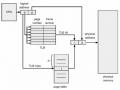
r
~ x
1
~ x
2
~ x
3
~ x
N T
Exclude stream 1
ZF 2 powder
Stream 2 Decoding
Exclude stream 1 , 2
Stream 3 Decoding
ZF 3 powder
Exclude streams 1, 2, 3,…,N T -1
Decode N T stream
ZF N T Powder
Figure 3.11 is a schematic diagram of the Zero-forcing receiver combined with ZF-IC sequential noise cancellation.
ZF 1 powder
Stream 1 Decoding | ||
Figure 3.11. V-BLAST Zero-forcing Receiver The entire ZF algorithm cancels successively in the following optimal order: Start-up:
𝑟 1 = 𝑟
𝐺 = 𝐻 +
2
Repeat 𝑖 = 1 → 𝑁 𝑇
𝑘 1 = 𝑎𝑟𝑔 min‖(𝐺) 𝑗 ‖
𝑗
𝑊 ̃ 𝑘 1= (𝐺) 𝑘 1
𝑦 𝑘 1= 𝑊 ̃ 𝑘 1𝑟 𝑖
𝑥 𝑘 1 = 𝑄(𝑦 𝑘 𝑖 )
𝑟 𝑖+1 = 𝑟 𝑖 − 𝑥 𝑘 𝑖 (𝐻) 𝑘 𝑖
𝑘 ̅
𝐺 = 𝐻 +
𝑖
2
𝑘 𝑖+1 = 𝑎𝑟𝑔 min ‖(𝐺) 𝑗 ‖
𝑗∉{𝑘 1 ,𝑘 2 ,⋯,𝑘 𝑖 }
𝑖 → 𝑖 + 1
Receiver diagram using Zero Forcing algorithm to cancel consecutive interference in optimal order: The data transmission rate of the 𝑘th data stream according to Shannon's theorem will be:
𝐶 𝑘
= log 2
(1 + 𝑆𝑁𝑅 𝑘
) = log 2
(1 +𝑃 𝑘) bits/s/Hz (3.49)
𝑁 0 ‖𝑊 𝑘 ‖ 2
The transmission speed of the system will be:
𝐶 = ∑
𝑁 𝑇
𝑘=1
𝐶 𝑘
bits/s/Hz (3.50)
In a fast-fading environment, the channel will vary, since the maximum transmission rate of the channel will be averaged.
𝐶 𝑍 ̅𝐹
= 𝐸(𝐶) = 𝐸 (∑ 𝑁
log 2
(1 +𝑃 𝑘) ) bits/s/Hz (3.51)
𝑁 0 ‖𝑊 𝑘 ‖ 2
~ x
2
~ x
3
~ x
N T
Exclude 1st stream
Define flow
ZF receiver and decoder
Exclude stream 1 , 2
ZF receiver and decoder
Define flow
Exclude streams 1, 2, 3,…,N T -1
ZF receiver and decoder
𝑘=1
Define flow | ZF receiver and decoder | ||
r~ x1
Figure 3.12. V-BLAST Zero-forcing receiver in optimal order
When the signal-to-noise ratio is high, we can approximate 𝐶 𝑍𝐹 by the following expression:
𝐶 ≈ 𝑁 log
𝑆𝑁𝑅 + 𝐸 (∑ 𝑁
log ( 1
)) (3.52a)
𝑍𝐹
2 𝑁
𝑘=1
2 ‖𝑊 𝑘 ‖ 2
𝐶 ≈ 𝑁 log
𝑆𝑁𝑅 + 𝐸(∑ 𝑁
(‖𝑊 ‖ 2 )) (3.52b)
𝑍𝐹
2 𝑁
𝑘=1 𝑘
𝑘=1
In case of decoding with sequential noise cancellation:
𝐶 𝑍 ̅𝐹−𝐼𝐶
= 𝐸 (∑ 𝑁
log 2
(1 +𝑃 𝑘) ) (3.53)
𝑁 0 ‖𝑊 ̃ 𝑘 ‖ 2
2
When the signal-to-noise ratio (SNR) is high, 𝐶 𝑍 ̅ 𝐹 −𝐼𝐶 is approximated by the following expression:
𝐶 ≈ 𝑁 log 𝑆𝑁𝑅 + 𝐸 (∑ 𝑁
log (‖𝑊 ̃
‖ )) (3.54)
𝑍𝐹−𝐼𝐶 2 𝑁
3.4.2.3. Limitations of Zero-forcing
𝑘=1 2 𝑘
When the signal-to-noise ratio is high, white Gaussian noise is negligible, the data streams interfere with each other mainly and overwhelm the white Gaussian noise. After the received signal vector is projected onto the orthogonal subspace to eliminate the Inter-Stream Interference, the remaining noise is just white noise which occupies a negligible amount, the signal is then passed through the Matched-Filter. Because the Matched-Filter works very effectively when the SNR is high.
When the signal-to-noise ratio is low, white Gaussian noise dominates the data streams, similar to when operating at high SNR, the Zero-forcing receiver also eliminates crosstalk from the decoded data stream caused by other data streams, however, when considering the optimal decoding order, we know that the projection of the received signal vector onto the orthogonal subspace has the effect of amplifying white Gaussian noise (the main component causing interference to the decoded data stream when the SNR is low), although the Matched-filter works very effectively when there is no crosstalk, at this time the white Gaussian noise is amplified much more than before the projection, for this reason, the ZF receiver does not work effectively when the SNR is low.
For the receiver to work effectively, we must design the receiver to optimize the signal to interference ratio and white noise SINR (Signal to Interference plus Noise Ratio) regardless of low or high SNR. Since the Matched-Filter works well when there is no cross-stream interference, if we use another algorithm that reduces cross-stream interference but does not amplify white noise, and then use the Matched-Filter, we will get a signal with a better signal to interference ratio and white noise SINR for the ZF receiver at low SNR. The receiver that can optimize the trade-off between cross-stream interference and Gaussian background noise is the MMSE receiver.
3.4.3. V-BAST Minimum Mean-Squared Error receiver
When the SNR is high, the Minimum Mean-Squared Error (MMSE) receiver acts like a ZF, and when the SNR is low the receiver takes advantage of the Matched-Filter.
Consider the general received signal of the following form:
𝑦 = ℎ𝑥 + 𝑧 (3.55)
Where 𝑧 is a complex circular color noise with an invertible correlation matrix 𝐾 𝑧 , ℎ is any column vector and x is the unknown symbol to be estimated, assuming 𝑥 and 𝑧 are uncorrelated. We know that if the noise is white, the Matched-Filter is the optimal filter that will give the maximum output SNR, so for the case of color noise, we will flatten the color noise to white noise
𝑧
before passing the signal through the Matched-Filter. First y is multiplied by 𝑘 −1 ⁄ 2
to do
flat noise
In this case 𝑧̃ will be white noise.
𝑥 = 𝑘 −1 ⁄ 2 𝑧 (3.56)
𝑧
𝑘 −1 ⁄ 2 𝑦 = 𝑘 −1 ⁄ 2 ℎ𝑥 + 𝑧̃ (3.57)
With
𝑧 𝑧
𝑧
𝑘 −1 ⁄ 2 = 𝑈Λ 𝐻 𝑈 𝐻 (3.58)
Where 𝑈 and Λ are decomposed from 𝐾 𝑧 . Since 𝐾 𝑧 is invertible, 𝐾 𝑧 can be written as:
𝐾 𝑧 = 𝑈Λ𝑈 𝐻 (3.59)
Where 𝑈 is the rotation matrix (or identity matrix) and Λ is the diagonal matrix, the matrix Λ 1⁄2 is the square root of the matrix Λ .
Λ 1 0
0 Λ 2
Λ = [ ⋮ ⋮
0 0
⋯ 0
⋯ 0
⋱ ⋮
⋯ Λ N R
] (3.60)
Λ 1⁄2 =
√ Λ 1 0 ⋯ 0
0 √Λ 2 ⋯ 0
(3.61)
⋮ ⋮ ⋱ ⋮
[ 0 0
⋯ √ Λ N R ]
Then, the output signal 𝑘 −1 ⁄ 2 𝑦 will be projected in the direction ℎ𝑘 −1 ⁄ 2 by multiplying by
𝑧 𝑧
𝑥
(𝑘 −1 ⁄ 2 ℎ) 𝐻 .
(𝑘 −1 ⁄ 2 ℎ) 𝐻 𝑘 −1 ⁄ 2 𝑦 = (𝑘 −1 ⁄ 2 ℎ) 𝐻 𝑘 −1 ⁄ 2 ℎ𝑥 + (𝑘 −1 ⁄ 2 ℎ) 𝐻 𝑧̃ (3.62a)
𝑥 𝑧 𝑥 𝑧 𝑥
ℎ 𝐻 𝑘 −1 𝑦 = ℎ 𝐻 𝑘 −1 ℎ𝑥 + ℎ 𝐻 𝑘 −1 𝑧 (3.62b)
𝑧 𝑧
From the above expression, the MMSE receiver will be represented through the vector:
𝑧
𝑉 = 𝑘 −1 ℎ (3.63)
The signal x will be estimated by multiplying y by
𝑧
𝑉 ∗ = ℎ 𝐻 𝑘 −1 (3.64)
The signal is then passed through the Match-Filter.