Learn about synchronization techniques in OFDM and OFDMA systems - 2

PREFACE

Nowadays, the demand for wireless communication is increasing, especially for mobile communication systems due to its flexibility, elasticity, mobility and convenience. Current and future wireless communication systems increasingly require higher capacity, better reliability, more efficient use of bandwidth, and better resistance to interference. Traditional communication systems and old multiplexing methods are no longer able to meet the requirements of future systems. Frequency spectrum is an extremely important resource in wireless communication. Making full use of frequency spectrum is an urgent issue. A proposed solution is to use OFDM orthogonal multi-carrier multiplexing technique and OFDMA orthogonal multiplexing technique in wireless communication, contributing to creating a more complete wireless communication system. OFDM is a technological solution to overcome the disadvantages of low spectrum efficiency of previous mobile communication systems. OFDM uses the technique of generating orthogonal subcarriers to transmit data, which helps in optimal use of channel bandwidth.

In this project, we will learn about OFDM technique, OFDMA multiple access technique and apply those techniques to create a wireless communication system that has more advantages than the old systems.

With the basic knowledge acquired during my studies at the Vietnam-Korea Friendship Information Technology College, along with the guidance and help of teacher Nguyen Thi Huyen Trang , I chose the topic: " Research on synchronization techniques in OFDM and OFDMA systems ".

I would like to sincerely thank the teachers of Vietnam-Korea Friendship Information Technology College for teaching and guiding me during my studies at school. In particular, I would like to sincerely thank teacher Nguyen Thi Huyen Trang for her dedicated help and guidance during the process of implementing this project.

Due to limited time and knowledge, the project inevitably has many shortcomings. I hope to receive guidance and comments from teachers and friends. I hope that this topic will be further improved.

CHAPTER I. OVERVIEW OF RADIO COMMUNICATIONS

1.1.INTRODUCTION TO WIRELESS INFORMATION NETWORKS

(Channel model)

Source

Source encoding

(source coding)

Channel encoding

(channel coding )

Preparation

(modulation)

Radio channel

(channel )

Target signal

(Destination)

Source Code

(source decoding)

Channel decoding

(Channel Decoding)

Demodulation

(Demodulation)

Figure 1.1 Information system model

Figure 1.1 shows a simple model of a wireless communication system. The source is first source coded to reduce redundant information, then channel coded to prevent errors caused by the transmission channel. The signal after going through the channel code is modulated so that it can be transmitted over a long distance. The modulation levels must be suitable for the conditions of the transmission channel. After the signal is transmitted at the transmitter, the signal received at the receiver will go through the reverse steps of the transmitter to receive the original signal. The quality of the received signal depends on the quality of the transmission channel, different modulation and coding methods.

We will learn the basic concepts in radio communication.

Channel

A transmission channel is a medium that allows radio waves to propagate. The transmission medium can be indoors, outdoors, or reflected on the ionosphere. Depending on the transmission medium, the channel has different properties.

Baseband transmission and bandwidth transmission

Conventional radio transmission is performed in passband, meaning that the signal must be modulated with a high-frequency carrier wave before being transmitted.

Baseband transmission is a non-carrier transmission. Non-carrier signals cannot be transmitted over long distances due to high attenuation.

Carrier wave

The carrier wave is a high-frequency wave that is multiplied by a useful signal before being sent to the transmitting antenna. The carrier wave itself does not carry a useful signal. However, because the carrier wave has a high frequency, when transmitted in a radio environment, the useful signal modulated into it will be less attenuated and can be transmitted over long distances. At the receiving end, the useful signal can be recovered by separating it from the carrier wave. Depending on the transmission environment and the allowed frequency band, the carrier frequency value is selected. Usually, the carrier wave is the center wave of the allowed frequency band of the information system.

Radio Resource Management

Radio resources are the spectrum width available for transmission. The spectrum width available is limited. Meanwhile, any transmission system needs a minimum quality and the demand for increasingly high speed to meet complex services. The problem of radio resource management is how with a given fixed frequency band the system operates with the best quality and the highest data transmission rate. With higher quality and higher information transmission rate, the system is said to have high spectrum efficiency. The task of radio resource management is also to divide the available spectrum width for different information systems so that the systems have the highest spectrum efficiency. For multi-user systems, radio resource management is the division of the frequency width and multiple access control so that the system is optimized in terms of signal quality and spectrum.

1.2. RADIO COMMUNICATION SYSTEMS

Radio communication systems can be classified according to the service provided: radio and television systems. The services of the two systems are voice and image.

Wireless communication systems can be classified according to the transmission method as full-duplex (mobile) or half-duplex (walkie-talkie) transmission systems.

Can be classified according to the transmission medium as microwave information (requires line-of-sight transmission) and wireless computer network information (multipath reflection and short distance).

1.3. RADIO TRANSMISSION LOSS

We will study the main problems of radio transmission and the difficulties they cause in digital information transmission systems. Signals transmitted over mobile radio channels will be reflected, refracted, diffracted, scattered ... and thus cause multipath phenomenon. The effects of radio transmission such as path loss, flat fading, frequency selective fading, Doppler effect, multipath delay spread ... all limit the efficiency of radio communication.

1.3.1. Transmission loss

Average transmission loss occurs due to phenomena such as: expansion in all directions of the signal, absorption of the signal by water, leaves ... and reflection from the ground. Average transmission loss depends on the distance and varies very slowly even for subscribers moving at high speed. At the transmitting antenna, radio waves will be transmitted in all directions (i.e. the wave is expanded in a spherical shape). Even when we use a directional antenna to transmit the signal, the wave is also expanded in a spherical shape but the energy density will then be concentrated in a certain area designed by us. Therefore, the power density of the wave decreases proportionally to the area of ​​the sphere. In other words, the wave intensity decreases proportionally to the square of the distance. Equation (1.1) calculates the power received after transmitting through a distance R

P PGG

(1.1)

RTTR 4 R

_ P R : Received signal power (W)

_ P T : Transmit power (W)

_ GR : Receiving antenna gain (isotropic antenna)

_ G T : Transmit antenna gain

_ : wavelength of carrier wave

_ R: radio wave transmission radius

Let L pt be the attenuation coefficient due to transmission in free space:

L pt ( db )  P T ( db )  P R ( db )   10 lg( G T )  10 lg( G R )  20 lg( f )  20 lg( R )  47, 6( db )

(1.2)

In general, we can build a fairly accurate model for satellite communication lines and direct (unobstructed) communication lines such as short-range point-to-point microwave communication lines. However, because most terrestrial communication lines such as mobile communication, wireless LAN, the transmission environment is much more complex, creating models is also more difficult. For example, for UHF mobile radio transmission channels, when the free space condition is not satisfied, we have the following transmission loss formula:

L pt ( db )   10 lg( G T )  10 lg( G R )  20 lg( h BS )  20 lg( h MS )  40 lg( R )

(1.3)

With _ h BS , _ h MS << R is the height of the base station antenna BS (Base Station) and the mobile station antenna MS (Mobile Station).

1.3.2. Multipath fading

The radio transmission path from the transmitter to the receiver always has obstacles, which will cause fading effects. At that time, the signal will arrive at the receiver from many different paths and have different delays and gains, each path is a copy of the original signal.

There are three possible situations that can occur on a radio transmission line: reflection, scattering, and diffraction.

Reflection: when waves hit flat surfaces.

Scattering: when a wave hits an object with an uneven surface and these objects have a length comparable to the wavelength.

Diffraction: when a wave hits objects that are much larger than its wavelength.

When the wave collides with obstacles, it will create countless copies of the signal, some of which will reach the receiver. Because the copies reflect, scatter, and diffract on different objects and follow different paths:

- The times these copies arrive at the receiver will be different, i.e. the phase delay between these parts will be different.

- These copies will have different powers arriving at the receiver due to different attenuation, or different amplitudes of the components.

Scattering

LOS

Reflex

Diffraction

Play

Collect

Figure 1.2 Multipath phenomenon in wireless communication

The signal at the receiver is the sum of all these copies, depending on the amplitude and phase of the components we will get

- The received signal is enhanced when the copies are in phase. The enhancement here is not a stronger and better signal but a more distorted signal.

- The received signal is canceled or reduced compared to the original signal when the components are out of phase.

Fast fading and slow fading

We consider two types of fading in terms of time.

- Fast fading: caused by multi-path scattering in the area around the receiver. Signals traveling over different distances of each transmission line will have different transmission times. The intensity depends on the attenuation of that line. For fixed frequency signals, transmission delay will cause the signal phase rotation. Each signal will have a different phase rotation. These signals are added together at the receiver, causing enhanced or attenuated noise depending on whether the phase of the signals is in phase or out of phase.

- Slow fading: caused by obstructions from buildings and natural terrain. The change in transmission loss occurs when the distance is large (10-100 times the wavelength) and depends on the size of the obstacle. This change occurs slowly so it is called slow fading.

Frequency Selective Fading and Flat Fading

These are two types of fading in terms of frequency. Wavelength is inversely proportional to frequency and so for a fixed transmission line the phase will change with frequency. The transmission distance of each multipath component is different so the phase change will also be different.

Definition: Coherent bandwidth B C is the bandwidth ∆f when the envelope coefficient between two signals is half of its maximum value.

( B c , ) 

1

c

1  (2 B ) 2. ​2

 0.5

(1.4)

In which: δ: delay spread depending on the radio transmission environment. Coherent bandwidth:

B c 

1  1

2 6 

(1.5)

Some common values ​​of channel delay spread in different environments.

Table 1.1 Delay spread values ​​of some typical environments.

Environment

Delay spread
Inside the buildings	< 0.1μs
Outdoor	< 0.2μs
Suburban	0.5μs
Urban	3 μs

Maybe you are interested!

• Qos Assurance Methods for Multimedia Communications zt2i3t4l5ee zt2a3gs zt2a3ge zc2o3n4t5e6n7ts low. The EF PHB requires a sufficiently large number of output ports to provide low delay, low loss, and low jitter. EF PHBs can be implemented if the output port's bandwidth is sufficiently large, combined with small buffer sizes and other network resources dedicated to EF packets, to allow the router's service rate for EF packets on an output port to exceed the arrival rate λ of packets at that port. This means that packets with PHB EF are considered with a pre-allocated amount of output bandwidth and a priority that ensures minimum loss, minimum delay and minimum jitter before being put into operation. PHB EF is suitable for channel simulation, leased line simulation, and real-time services such as voice, video without compromising on high loss, delay and jitter values. Figure 2.10 Example of EF installation Figure 2.10 shows an example of an EF PHB implementation. This is a simple priority queue scheduling technique. At the edges of the DS domain, EF packet traffic is prioritized according to the values ​​agreed upon by the SLA. The EF queue in the figure needs to output packets at a rate higher than the packet arrival rate λ. To provide an EF PHB over an end-to-end DS domain, bandwidth at the output ports of the core routers needs to be allocated in advance to ensure the requirement μ > λ. This can be done by a pre-configured provisioning process. In the figure, EF packets are placed in the priority queue (the upper queue). With such a length, the queue can operate with μ > λ. Since EF was primarily used for real-time services such as voice and video, and since real-time services use UDP instead of TCP, RED is generally not suitable for EF queues because applications using UDP will not respond to random packet drop and RED will strip unnecessary packets. 2.2.4.2 Assured Forwarding (AF) PHB PHB AF is defined by RFC 2597. The purpose of PHB AF is to deliver packets reliably and therefore delay and jitter are considered less important than packet loss. PHB AF is suitable for non-real-time services such as applications using TCP. PHB AF first defines four classes: AF1, AF2, AF3, AF4. For each of these AF classes, packets are then classified into three subclasses with three distinct priority levels. Table 2.8 shows the four AF classes and 12 AF subclasses and the DSCP values ​​for the 12 AF subclasses defined by RFC 2597. RFC 2597 also allows for more than three separate priority levels to be added for internal use. However, these separate priority levels will only have internal significance. PHB Class PHB Subclass Package type DSCP AF4 AF41 Short 100010 AF42 Medium 100100 AF43 High 100110 AF3 AF31 Short 011010 AF32 Medium 011100 AF33 High 011110 AF2 AF21 Short 010010 AF22 Medium 010100 AF23 High 010110 AF1 AF11 Short 001010 AF12 Medium 001100 AF13 High 001110 Table 2.8 AF DSCPs The AF PHB ensures that packets are forwarded with a high probability of delivery to the destination within the bounds of the rate agreed upon in an SLA. If AF traffic at an ingress port exceeds the pre-priority rate, which is considered non-compliant or “out of profile”, the excess packets will not be delivered to the destination with the same probability as the packets belonging to the defined traffic or “in profile” packets. When there is network congestion, the out of profile packets are dropped before the in profile packets are dropped. When service levels are defined using AF classes, different quantity and quality between AF classes can be realized by allocating different amounts of bandwidth and buffer space to the four AF classes. Unlike EF, most AF traffic is non-real-time traffic using TCP, and the RED queue management strategy is an AQM (Adaptive Queue Management) strategy suitable for use in AF PHBs. The four AF PHB layers can be implemented as four separate queues. The output port bandwidth is divided into four AF queues. For each AF queue, packets are marked with three “colors” corresponding to three separate priority levels. In addition to the 32 DSCP 1 groups defined in Table 2.8, 21 DSCPs have been standardized as follows: one for PHB EF, 12 for PHB AF, and 8 for CSCP. There are 11 DSCP 1 groups still available for other standards. 2.2.5.Example of Differentiated Services We will look at an example of the Differentiated Service model and mechanism of operation. The architecture of Differentiated Service consists of two basic sets of functions: Edge functions: include packet classification and traffic conditioning. At the inbound edge of the network, incoming packets are marked. In particular, the DS field in the packet header is set to a certain value. For example, in Figure 2.12, packets sent from H1 to H3 are marked at R1, while packets from H2 to H4 are marked at R2. The labels on the received packets identify the service class to which they belong. Different traffic classes receive different services in the core network. The RFC definition uses the term behavior aggregate rather than the term traffic class. After being marked, a packet can be forwarded immediately into the network, delayed for a period of time before being forwarded, or dropped. We will see that there are many factors that affect how a packet is marked, and whether it is forwarded immediately, delayed, or dropped. Figure 2.12 DiffServ Example Core functionality: When a DS-marked packet arrives at a Diffservcapable router, the packet is forwarded to the next router based on Per-hop behavior is associated with packet classes. Per-hop behavior affects router buffers and the bandwidth shared between competing classes. An important principle of the Differentiated Service architecture is that a router's per-hop behavior is based only on the packet's marking or the class to which it belongs. Therefore, if packets sent from H1 to H3 as shown in the figure receive the same marking as packets from H2 to H4, then the network routers treat the packets exactly the same, regardless of whether the packet originated from H1 or H2. For example, R3 does not distinguish between packets from h1 and H2 when forwarding packets to R4. Therefore, the Differentiated Service architecture avoids the need to maintain router state about separate source-destination pairs, which is important for network scalability. Chapter Conclusion Chapter 2 has presented and clarified two main models of deploying and installing quality of service in IP networks. While the traditional best-effort model has many disadvantages, later models such as IntServ and DiffServ have partly solved the problems that best-effort could not solve. IntServ follows the direction of ensuring quality of service for each separate flow, it is built similar to the circuit switching model with the use of the RSVP resource reservation protocol. IntSer is suitable for services that require fixed bandwidth that is not shared such as VoIP services, multicast TV services. However, IntSer has disadvantages such as using a lot of network resources, low scalability and lack of flexibility. DiffServ was born with the idea of ​​solving the disadvantages of the IntServ model. DiffServ follows the direction of ensuring quality based on the principle of hop-by-hop behavior based on the priority of marked packets. The policy for different types of traffic is decided by the administrator and can be changed according to reality, so it is very flexible. DiffServ makes better use of network resources, avoiding idle bandwidth and processing capacity on routers. In addition, the DifServ model can be deployed on many independent domains, so the ability to expand the network becomes easy. Chapter 3: METHODS TO ENSURE QoS FOR MULTIMEDIA COMMUNICATIONS In packet-switched networks, different packet flows often have to share the transmission medium all the way to the destination station. To ensure the fair and efficient allocation of bandwidth to flows, appropriate serving mechanisms are required at network nodes, especially at gateways or routers, where many different data flows often pass through. The scheduler is responsible for serving packets of the selected flow and deciding which packet will be served next. Here, a flow is understood as a set of packets belonging to the same priority class, or originating from the same source, or having the same source and destination addresses, etc. In normal state when there is no congestion, packets will be sent as soon as they are delivered. In case of congestion, if QoS assurance methods are not applied, prolonged congestion can cause packet drops, affecting service quality. In some cases, congestion is prolonged and widespread in the network, which can easily lead to the network being "frozen", or many packets being dropped, seriously affecting service quality. Therefore, in this chapter, in sections 3.2 and 3.3, we introduce some typical network traffic load monitoring techniques to predict and prevent congestion before it occurs through the measure of dropping (removing) packets early when there are signs of impending congestion. 3.1. DropTail method DropTail is a simple, traditional queue management method based on FIFO mechanism. All incoming packets are placed in the queue, when the queue is full, the later packets are dropped. Due to its simplicity and ease of implementation, DropTail has been used for many years on Internet router systems. However, this algorithm has the following disadvantages: − Cannot avoid the phenomenon of “Lock out”: Occurs when 1 or several traffic streams monopolize the queue, making packets of other connections unable to pass through the router. This phenomenon greatly affects reliable transmission protocols such as TCP. According to the anti-congestion algorithm, when locked out, the TCP connection stream will reduce the window size and reduce the packet transmission speed exponentially. − Can cause Global Synchronization: This is the result of a severe “Lock out” phenomenon. Some neighboring routers have their queues monopolized by a number of connections, causing a series of other TCP connections to be unable to pass through and simultaneously reducing the transmission speed. After those monopolized connections are temporarily suspended, Once the queue is cleared, it takes a considerable amount of time for TCP connections to return to their original speed. − Full Queue phenomenon: Data transmitted on the Internet often has an explosion, packets arriving at the router are often in clusters rather than in turn. Therefore, the operating mechanism of DropTail makes the queue easily full for a long period of time, leading to the average delay time of large packets. To avoid this phenomenon, with DropTail, the only way is to increase the router's buffer, this method is very expensive and ineffective. − No QoS guarantee: With the DropTail mechanism, there is no way to prioritize important packets to be transmitted through the router earlier when all are in the queue. Meanwhile, with multimedia communication, ensuring connection and stable speed is extremely important and the DropTail algorithm cannot satisfy. The problem of choosing the buffer size of the routers in the network is to “absorb” short bursts of traffic without causing too much queuing delay. This is necessary in bursty data transmission. The queue size determines the size of the packet bursts (traffic spikes) that we want to be able to transmit without being dropped at the routers. In IP-based application networks, packet dropping is an important mechanism for indirectly reporting congestion to end stations. A solution that prevents router queues from filling up while reducing the packet drop rate is called dynamic queue management. 3.2. Random elimination method – RED 3.2.1 Overview RED (Random Early Detection of congestion; Random Early Drop) is one of the first AQM algorithms proposed in 1993 by Sally Floyd and Van Jacobson, two scientists at the Lawrence Berkeley Laboratory of the University of California, USA. Due to its outstanding advantages compared to previous queue management algorithms, RED has been widely installed and deployed on the Internet. The most fundamental point of their work is that the most effective place to detect congestion and react to it is at the gateway or router. Source entities (senders) can also do this by estimating end-to-end delay, throughput variability, or the rate of packet retransmissions due to drop. However, the sender and receiver view of a particular connection cannot tell which gateways on the network are congested, and cannot distinguish between propagation delay and queuing delay. Only the gateway has a true view of the state of the queue, the link share of the connections passing through it at any given time, and the quality of service requirements of the traffic flows. The RED gateway monitors the average queue length, which detects early signs of impending congestion (average queue length exceeding a predetermined threshold) and reacts appropriately in one of two ways: − Drop incoming packets with a certain probability, to indirectly inform the source of congestion, the source needs to reduce the transmission rate to keep the queue from filling up, maintaining the ability to absorb incoming traffic spikes. − Mark “congestion” with a certain probability in the ECN field in the header of TCP packets to notify the source (the receiving entity will copy this bit into the acknowledgement packet). Figure 3. 1 RED algorithm The main goal of RED is to avoid congestion by keeping the average queue size within a sufficiently small and stable region, which also means keeping the queuing delay sufficiently small and stable. Achieving this goal also helps: avoid global synchronization, not resist bursty traffic flows (i.e. flows with low average throughput but high volatility), and maintain an upper bound on the average queue size even in the absence of cooperation from transport layer protocols. To achieve the above goals, RED gateways must do the following: − The first is to detect congestion early and react appropriately to keep the average queue size small enough to keep the network operating in the low latency, high throughput region, while still allowing the queue size to fluctuate within a certain range to absorb short-term fluctuations. As discussed above, the gateway is the most appropriate place to detect congestion and is also the most appropriate place to decide which specific connection to report congestion to. − The second thing is to notify the source of congestion. This is done by marking and notifying the source to reduce traffic. Normally the RED gateway will randomly drop packets. However, if congestion If congestion is detected before the queue is full, it should be combined with packet marking to signal congestion. The RED gateway has two options: drop or mark; where marking is done by marking the ECN field of the packet with a certain probability, to signal the source to reduce the traffic entering the network. − An important goal that RED gateways need to achieve is to avoid global synchronization and not to resist traffic flows that have a sudden characteristic. Global synchronization occurs when all connections simultaneously reduce their transmission window size, leading to a severe drop in throughput at the same time. On the other hand, Drop Tail or Random Drop strategies are very sensitive to sudden flows; that is, the gateway queue will often overflow when packets from these flows arrive. To avoid these two phenomena, gateways can use special algorithms to detect congestion and decide which connections will be notified of congestion at the gateway. The RED gateway randomly selects incoming packets to mark; with this method, the probability of marking a packet from a particular connection is proportional to the connection's shared bandwidth at the gateway. − Another goal is to control the average queue size even without cooperation from the source entities. This can be done by dropping packets when the average size exceeds an upper threshold (instead of marking it). This approach is necessary in cases where most connections have transmission times that are less than the round-trip time, or where the source entities are not able to reduce traffic in response to marking or dropping packets (such as UDP flows). 3.2.2 Algorithm This section describes the algorithm for RED gateways. RED gateways calculate the average queue size using a low-pass filter. This average queue size is compared with two thresholds: minth and maxth. When the average queue size is less than the lower threshold, no incoming packets are marked or dropped; when the average queue size is greater than the upper threshold, all incoming packets are dropped. When the average queue size is between minth and maxth, each incoming packet is marked or dropped with a probability pa, where pa is a function of the average queue size avg; the probability of marking or dropping a packet for a particular connection is proportional to the bandwidth share of that connection at the gateway. The general algorithm for a RED gateway is described as follows: [5] For each packet arrival Caculate the average queue size avg If minth ≤ avg < maxth div.maincontent .s1 { color: black; font-family:"Times New Roman", serif; font-style: normal; font-weight: normal; text-decoration: none; font-size: 15pt; } div.maincontent .s2 { color: black; font-family:"Times New Roman", serif; font-style: normal; font-weight: bold; text-decoration: none; font-size: 15pt; } div.maincontent .p { color: black; font-family:"Times New Roman", serif; font-style: normal; font-weight: normal; text-decoration: none; font-size: 14pt; margin:0pt; } div.maincontent p { color: black; font-family:"Times New Roman", serif; font-style: normal; font-weight: normal; text-decoration: none; font-size: 14pt; margin:0pt; } div.maincontent .s3 { color: black; font-family:"Times New Roman", serif; font-style: normal; font-weight: bold; text-decoration: none; font-size: 14pt; } div.maincontent .s4 { color: black; font-family:"Times New Roman", serif; font-style: normal; font-weight: normal; text-decoration: none; font-size: 14pt; } div.maincontent .s5 { color: black; font-family:"Times New Roman", serif; font-style: italic; font-weight: normal; text-decoration: none; font-size: 14pt; } div.maincontent .s6 { color: black; font-family:"Times New Roman", serif; font-style: italic; font-weight: bold; text-decoration: none; font-size: 14pt; } div.maincontent .s7 { color: black; font-family:Wingdings; font-style: normal; font-weight: normal; text-decoration: none; font-size: 14pt; } div.maincontent .s8 { color: black; font-family:Arial, sans-serif; font-style: italic; font-weight: bold; text-decoration: none; font-size: 15pt; } div.maincontent .s9 { color: black; font-family:"Times New Roman", serif; font-style: normal; font-weight: bold; text-decoration: none; font-size: 14pt; } div.maincontent .s10 { color: black; font-family:"Times New Roman", serif; font-style: normal; font-weight: normal; text-decoration: none; font-size: 9pt; vertical-align: 6pt; } div.maincontent .s11 { color: black; font-family:"Times New Roman", serif; font-style: normal; font-weight: normal; text-decoration: none; font-size: 13pt; } div.maincontent .s12 { color: black; font-family:"Times New Roman", serif; font-style: normal; font-weight: normal; text-decoration: none; font-size: 10pt; } div.maincontent .s13 { color: black; font-family:"Times New Roman", serif; font-style: normal; font-weight: normal; text-d
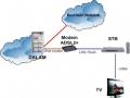• Learn about IPTV technology and implementation solutions at VNPT Bac Ninh - 9
• Corresponding Techniques for Task Type T 1 Μ , T 1 P , T 1  2
• Learn active learning methods and apply them to spam filtering problems - 1
• Learn about HSDPA technology and its application to 3rd - 6th generation mobile networks

For each environment with different delay spread, we will calculate the corresponding Coherent bandwidth.

- Frequency selective fading: if the bandwidth of the modulated signal is much larger than the Coherent bandwidth of the channel, different frequency components of the signal have different fading characteristics. Frequency selective channels are called time-dispersive channels. Besides the amplitude, the shape of the pulse is also changed. That is, the signal transmitted through this channel will be severely distorted.

- Flat fading: the bandwidth of the modulated signal is smaller than the Coherent bandwidth of the channel, all frequency components of the signal have the same fading characteristics. With flat fading, only the amplitude of the pulse changes. Every radio channel

It is impossible for a channel to have a flat response over the entire radio frequency range. However, the channel can be considered flat over a small frequency range.

Figure 1.3 is an example of the response of a frequency selective channel. It can be seen that at different frequencies the signal will be affected by both amplitude and phase, and therefore it will be difficult to recover the data exactly as it was originally.

Frequency selective fading is a difficult problem to predict when transmitting radio signals. It causes linear distortion. However, with OFDM technology, by dividing the signal into many subcarriers for transmission, each subcarrier occupies only a narrow frequency band enough to satisfy the frequency selective fading and only flat fading, this problem is easily solved.

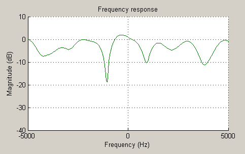
Figure 1.3 Response of frequency selective fading channel

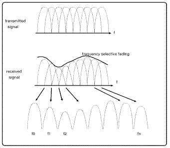
Figure 1.4 Effect of frequency selective fading channel