a. Forecasts: (Constant), SI, PE, FC, EE
b. Dependent variable: UIE |
Maybe you are interested!
-
 Testing for Violations of Regression Assumptions
 -
 Tests in Binary Logistic Regression Models
 -
 Hypothesis Testing About the Significance of Regression Coefficients
 -
 Measurement Indicators of Variables in Regression Models
 -
 Results of Testing Cronbach's Alpha Coefficient of Independent Variable
Table 4.8. Parameter table of linear regression model
Model
Unstandardized coefficient | Standardization factor | t | Sig. | Multicollinearity statistics | ||||
B | Standard error | Beta | Tolerance | VIF | ||||
1 | (Constant) | -.327 | .169 | -1.930 | .055 | |||
PE | .224 | .046 | .205 | 4,866 | .000 | .699 | 1,431 | |
EE | .494 | .049 | .467 | 10,180 | .000 | .586 | 1,707 | |
FC | .271 | .048 | .239 | 5,682 | .000 | .700 | 1,429 | |
SI | .128 | .038 | .136 | 3.353 | .001 | .746 | 1,340 | |
a. Dependent variable: UIE
As the results presented in Table 4.8, all four impact components have a significant influence on customers' intention to use the service, with a significance level of sig < 0.05.
To determine the level of influence of independent variables on the dependent variable Intention to use, we can base on the Beta coefficient. If the absolute value of the Beta coefficient of a factor is larger, the factor has a more important influence on Intention to use. Looking at equation 4.1, we see that Expected Effort (EE) has the strongest influence on Intention to use (UIE) because Beta equals 0.467, the largest among Betas, followed by customers' perception of Convenience (Beta equals 0.239). The factor with the next level of influence
is Expected Performance (PE) with Beta of 0.205. Finally, customer perception of Social Influence (SI) with Beta of 0.136.
4.4.3. Testing the assumptions of the regression model
From the results of observations in the sample, we must generalize the conclusions for the relationship between variables in the population. Acceptance and interpretation of regression results cannot be separated from the necessary assumptions of the regression model. If the assumptions are violated, the estimated results are no longer reliable (Hoang Trong and Chu Nguyen Mong Ngoc, 2005).
The assumptions of linear regression include:
- No multicollinearity.
- The variance of the residual is constant.
- The residuals are normally distributed.
- There is no correlation between the residuals.
a. Consider the assumption that there is no multicollinearity.
In the multiple linear regression model, it is assumed that there is no multicollinearity between the independent variables of the model. This phenomenon can be detected through the magnification factor (VIF). Normally, the acceptable level is the VIF value ≤ 10. If the VIF is greater than 10, there is a serious multicollinearity phenomenon (Hair, 2010). In this model, in order to not have a serious multicollinearity phenomenon, the VIF must be less than 10. Through Table 4.8, the component VIF values are all less than 10, indicating that there is no multicollinearity phenomenon.
b. Assume the variance of the residuals is constant.
Based on the graph of the standardized residuals against the predicted value of the dependent variable, the Intention is used to check whether there is a phenomenon of heteroscedasticity. Observing the scatter plot in Figure 4.1, it can be seen that the residuals are randomly scattered along the zero abscissa. Thus, the variance of the residuals remains constant.
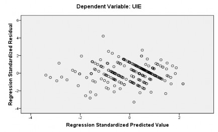
Figure 4.1. Scatter plot
c. Assumption of normal distribution of residuals
The residuals may not follow the normal distribution for many reasons, using the wrong model, the variance is not constant, the number of residuals is not large enough for analysis (Hoang Trong & Chu Nguyen Mong Ngoc, 2005). In this section, the author uses the Histogram and PP charts for consideration. Looking at Chart 4.2 and Chart 4.3, the assumption of normal distribution of the residuals is not violated.
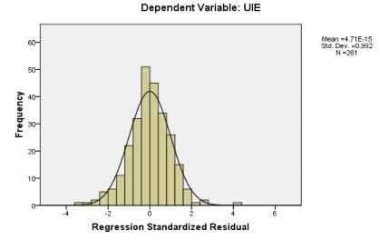
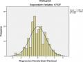
Figure 4.2. Frequency histogram of standardized residuals
Considering the frequency of standardized residuals in Figure 4.2, the residual distribution is approximately normal St.Dev = 0.99, which is close to 1. Therefore, it can be concluded that the normal distribution hypothesis is not violated.
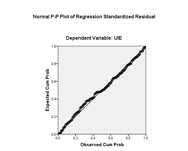
Figure 4.3. PP frequency chart
From Figure 4.3, the observation points are not scattered too far from the expected line but are scattered along and close to the expected line, so the hypothesis that the distribution of the residuals is normally distributed can be accepted. From the above test results, it can be concluded that the normal distribution assumption is not violated.
d. Assumption of independence of residuals
When autocorrelation occurs, the estimates of the regression model are unreliable. The test method to detect autocorrelation is the Dubin-Watson (d) test. If 1 < d < 3, the model is concluded to have no autocorrelation, if 0 < d < 1, the model is concluded to have positive autocorrelation, if 3 < d < 4, the model is concluded to have negative autocorrelation. Table 4.6 shows that Durbin-Watson is 2.009, which means that the assumption of no correlation between the residuals is accepted.
Thus, the assumptions of the linear regression model are all satisfied.
4.4.4. Testing research hypotheses
Five research hypotheses have been proposed (see section 2.4). Regression analysis shows that four factors extracted from EFA have a significant impact on customers' intention to use the service. The individual regression coefficients in the model are used to test the important role of the independent variables in influencing the dependent variable. The individual coefficients (unstandardized) in the model indicate the level of influence of the variables, specifically as follows:
Expected Effort is the factor that has the greatest influence on customers' intention to use the service (has the largest regression coefficient). The positive sign of the Beta coefficient means that the relationship between the factor "Expected Effort" and "Intention to use" is a positive relationship. Accordingly, when customers feel that the expected effort is higher, the intention to use increases. The regression result (Table 4.8) shows that EE has Beta = 0.494 (significance level < 0.05), which means that when Expected Effort increases by 1 standard deviation unit, the intention to use increases by 0.494 standard deviation units. Therefore, hypothesis H 2 is accepted.
Convenience is the next most influential factor on customers' intention to use. The positive sign of the Beta coefficient means that the relationship between the factor "Convenience" and "Intention to use" is in the same direction. Accordingly, when customers
Customers find that the more convenient the service conditions are, the more they intend to use the service. The regression results (Table 4.8) show that FC has Beta = 0.271 (significance level < 0.05), which means that when the Convenience Conditions increase by 1 standard deviation unit, the Intention to use increases by 0.271 standard deviation units. So hypothesis H 3 is accepted.
Expected effectiveness is the next factor that has the greatest influence on customers' intention to use. The positive sign of the Beta coefficient means that the relationship between the factor "Expected effectiveness" and "Intention to use" is a positive relationship. Accordingly, when customers feel that the expected effectiveness is higher, the intention to use increases. The regression result (Table 4.8) shows that PE has Beta = 0.224 (significance level < 0.05), which means that when Expected effectiveness increases by 1 standard deviation unit, the intention to use increases by 0.224 standard deviation units. Therefore, hypothesis H 1 is accepted.
Social influence is the factor that has the least influence on customers' intention to use in the model. The positive sign of the Beta coefficient means that the relationship between the factor "Social influence" and "Intention to use" is a positive relationship. Accordingly, when customers feel that the social influence of using ebanking services is higher, the intention to use increases. The regression result (Table 4.8) shows that SI has Beta = 0.128 (significance level < 0.05), which means that when Security increases by 1 standard deviation unit, the intention to use increases by 0.128 standard deviation units. So hypothesis H 4 is accepted.
With 85% confidence, Risk Perception is a factor that affects customers' Intention to Use. The negative sign of the Beta coefficient means that the relationship between the factor "Risk Perception" and "Intention to Use" is an inverse relationship. Accordingly, the higher the customer's risk perception, the lower the Intention to Use. However, because this factor only reaches 85% confidence, the author does not include this factor in the regression model. Thus, at 95% confidence, the hypothesis H 5 is rejected.
In summary, the research hypotheses have the following test results (Table 4.9):
Table 4.9. Results of testing research hypotheses
Hypothesis
Stated | Statistical value | Result | |
H 1 | Expected positive impact on Italy customer's intention to use ebanking services. | 0.000 < 0.05 | Accept |
H 2 | Effort expectancy positively affects Intention use of customer ebanking services. | 0.000 < 0.05 | Accept |
H 3 | Favorable conditions positively impact Italy customer's intention to use ebanking services. | 0.000 < 0.05 | Accept |
H 4 | Social influence positively affects Intention use of customer ebanking services. | 0.000 < 0.05 | Accept |
H 5 | Risk Perception Has a Negative Impact on Intention use of customer ebanking services. | 0.128 > 0.05 | Reject |
4.5. ANALYSIS OF THE IMPACT OF QUALITATIVE VARIABLES ON THE INTENTION TO USE EBANKING SERVICE
4.5.1. Gender
Table 4.10. T-test results for gender
Group statistics
Gender *
N | Medium | Standard deviation | Mean standard deviation | ||
UIE | 0 | 116 | 3.3851 | .85534 | .07942 |
1 | 145 | 3.4575 | .80789 | .06709 |
* 0: Female; 1: Male
Levene's test for equality of variances | T-test for equality of means | |||||
F | Sig. | t | df | Sig. (2- tailed) | ||
UIE | Equal variance | .104 | .747 | -.701 | 259 | .484 |
Different variance | -.697 | 240,072 | .487 | |||
The significance level of Levene's Test is 0.747 (> 0.05), meaning that the variance of the two groups is equal, from which we can see that the significance level of T-test is 0.484> 0.05, showing that there is no difference between men and women in their intention to use ebanking services.
4.5.2. Age
To test the difference in usage intention between customer groups of different ages, the author conducted an ANOVA test. The results of the ANOVA test are presented in the following table.
Table 4.11. ANOVA test results by age
Descriptive statistics
UIE* | ||||||||
N | Medium | Standard deviation | Standard error | 95% Confidence Interval of Mean | Minimum | Maximum | ||
Lower limit | Upper limit | |||||||
0 | 177 | 3.4652 | .79388 | .05967 | 3.3474 | 3.5829 | 1.00 | 5.00 |
1 | 70 | 3.3952 | .91206 | .10901 | 3.1778 | 3.6127 | 1.00 | 5.00 |
2 | 14 | 3.0714 | .78641 | .21018 | 2.6174 | 3.5255 | 1.33 | 4.00 |
3 | 0 | 0 | 0 | 0 | 0 | 0 | 0 | 0 |
Total | 261 | 3.4253 | .82848 | .05128 | 3.3243 | 3.5263 | 1.00 | 5.00 |
*0: 18 - 30; 1: 31 - 40; 2: 41 - 50; 3: Over 50