Steps to Solve Two-Variable Quadratic Problems Using Geometric Methods

1, r

where r is the number of constraints to be added

(false). In the objective function f(x) min coefficient of the unknowns x n +k is M (where M is an arbitrarily large number, larger than any constant to be compared with it); in the objective function f(x) The max coefficient of the unknowns x n +k is -M.

This newly obtained problem is called the extension problem , denoted by ( P M ).

Example 6Put the following problem into standard form (problem ( P )): (1) f(x) = 2x 1+3x 2+ x 3 + x 4min(max)



 x 1

(2) 





5x2​

4x2​

3x2​

x 3

5x4​

6x4​

8x4​

25

 18

28

(3) x 1 0 , x 2 0, x 3 0, x 4 0

Prize

First, we change the signs of both sides of the second constraint. The first constraint already has a basic variable x 1 , so we only need to add a dummy variable x 5into the second constraint and the pseudo- x 6on the third constraint. We get the extended problem (P M ):

(1') f M (x M ) = 2x 1 +3x 2 + x 3 + x 4 M(x 5 +x 6 ) min(max)

(2')

 x 1





5x2​

4x2​

x 3

5x4​

6x4​

x 5

25

18



  3x 2

8x4​

x 6 28

(3') x 1 0 , x 2 0, x 3 0, x 4 0, x 5 0, x 6 0

Example 7Put the following problem into standard form (problem ( P )):

n

(1) f(x) =  c j x j

j  1

min ( max)

n

(2)  a i j x jb i

j  1

, with b i 0 ( i = 1, m )

(3) x j 0 , j = 1, 2, …, n

Prize

Adding to the left side of each constraint in (2) an unknown we get the expanded problem

n

(P M ): (1') f M (x M ) =  c j x j

j  1

M(x n+1 +...+x n+m ) min ( max)

n

(2')  a i j x j+ x n +k b i

j  1

, with b i 0 ( i = 1, m , k = 1, m )

(3') x j 0 , j = 1, 2, …, n, n+1,..., n+m.

Comment:

i) If x = (x 1 ,..., x n ) is a solution to problem ( P ) then x M= (x 1 ,...,x n ,0,...,0) is a solution to the extended problem (P M ).

ii) If x *= ( x *,..., x *,0,...,0) is the PATU of the extended problem (P M ) then

M 1 n

x *= ( x *,..., x *) is the PATU of the problem ( P ). Conversely, if x *= ( x *,..., x *) To be

1 n 1 n

The PATU of problem ( P ) is x *= ( x *,..., x *,0,...,0) is the PTU of the open problem

M 1 n

wide (P M ). Therefore, if (P M ) does not have PATU, then ( P ) does not have PATU either.

iii) If (P M ) has PATU x * = ( x * ,..., x * , x *

,..., x *

), with at least one pseudonym

M 1 n

n  1

n  m

x

* n  k

> 0 then ( P ) does not have PA. Indeed, suppose on the contrary ( P ) has PA as

M

x = (x 1 ,..., x n ). Then (P M ) has PA as x M= (x 1 ,...,x n ,0,...,0); moreover because M is large

x

optional and

* n  k

> 0 so f M (x M ) < f M ( x *

) for the case f min and f M (x M )

M

> f M ( x *) for the case f max . This makes no sense given the optimal nature of

x

.

* M

Conclude

Any canonical QHTT problem can be reduced to a standard QHTT problem.

If the extended problem (P M ) does not have PATU, then problem ( P ) does not have PATU.

If the extended problem (P M ) has PATU and all the pseudo-variables are 0, then removing the pseudo-variables we get the PATU of the problem ( P ).

If the extended problem (P M ) has PATU and at least one nonzero pseudo-variable, then the problem ( P ) has no PA and therefore no PATU.

In short , every general QHTT problem can be reduced to a canonical QHTT problem; every canonical QHTT problem can be reduced to a standard QHTT problem. Thus, we only need to solve the standard problem.

2.4. Properties of the QHTT problem

Property 1 : (existence of alternatives)

If the problem has a solution, there is a basic solution.

Property 2 : (existence of optimal solutions)

If the problem has an optimal solution, then there is an optimal basic solution.

Property 3 : (finiteness of the number of options)

The number of different basic solutions in each problem is finite.

................................................................ ................................................................ .........

Exercise

Lesson 1.19In problems 1 through 6 below: 1. (1) f(x) = 2x 1+3x 2+ x 3 + x 4max



 x 1

(2) 



 x 1

x 2

x 2

x 2

2x3​

x 3

2x3​

x 4

2x4​

x 4

x 5

32

16

32

(3) x 1 , x 3 0; x 2 0; x 4 , x 5 optional

2. (1) f(x) = 2x 1 +3x 2 + x 3 + x 4 min

2x 1

(2) 4x

x 2

2x

3x3​

x

4x5​

5x

17

20

1 3 4 5



 2x 1 4x 5 x 6 6

(3) x j 0 (j = 1.6 )

3. (1) f(x) = 2x 1 +3x 2 + x 3 + x 4 max

x 1

(2) x

x 2

2x

2x3​

x x

5

15

1 2 3 4



 2x 1 x 2 3x 3 8

(3) x j 0 (j = 1.4 )

4. (1) f(x) = 2x 1 +3x 2 + x 3 + x 4 min

x 1

(2) x

2x2​

2x

2x3​

x

 7

15

2 3 4



 2x 1 3x 3 x 4 8

(3) x j 0 (j = 1.4 )

5.

(1) f(x) = - 2x 1 + x 2 + x 4 min

x 1

(2) x

x 2

x

x 3

x x

15

27

1 2 3 4



 2x 1 x 2 x 3

18

(3) x j 0 (j = 1.4 )

6.

(1) f(x) = x 1 + 2x 2 – x 3 max

 4x 1

(2) x

4x2​

x

2x3​

2x

 6

6

1 2 3



 2x 1 x 2 2x 3 4

(3) x j 0 ( j = 1.3 )

a) Which problems have a canonical form?

b) Which problems have standard form? If the problem has standard form, indicate the basic variables and their order? Find its initial basic solution.

c) For any problem that does not have a standard form, put it into standard form and then tell which is the fundamental unknown, what is the fundamental unknown (main unknown? auxiliary unknown? pseudo unknown?), what is its order? What is the initial basic solution of this standard form problem?

3. SUMMER STUDY METHOD

3.1. Some results in geometry

The line ax + by = c divides the Oxy plane into two regions: One region consists of all points (x,y) satisfying the inequality ax + by > c; one region consists of all points (x,y) satisfying the inequality ax + by < c. Thus, each inequality of the form ax + by c ( or ax + by c, with the condition a 2 +b 20) defines a closed half plane.

The family of lines ax + by = m ( m   ) is a set of parallel lines, which we call level lines (corresponding to level m ). If we translate one



straight line in the family (a level line) in the direction of vector n = (a;b) then the value

the corresponding value of m increases, and in the opposite direction the corresponding value of m decreases.

3.2. Steps to solve two-variable quadratic equations using geometric methods

Solve the problem: f(x) = c 1 x 1+ c 2 x 2min ( max) (1)

 ax  ax

  b , i 1, m

(2)

D: 

i1 1

i2 2 i

  

  x 10 , x 20 (or

a x 1 b , c x 2 d)

(3)

Step 1Draw the constraint region D in the Ox 1 x 2 plane .

Step 2Determine point C(c 1 ,c 2 ); draw OC or unit vector





n in the same direction OC =

(c 1 ,c 2 ); draw a level line (d) n and cut the domain of option D.

Step 3

 To find the optimal solution for the problem f  max , we translate the level curve (d)



in the direction of vector n until further translation causes the level curve to become

If there are any points in common with D, then stop. The point belonging to D lying on this final level line ( this is the point of contact of (d) with D and there can be many points ) is PATU and the value of the objective function at that point is the optimal value of the problem.

 To find the optimal solution for the problem f  min , we translate the level curve (d)



in the opposite direction of vector n until the next translation makes

The level curve no longer has common points with D, then stop. The point belonging to D on this last level curve ( this is the contact point of (d) with D and there can be many points ) is the PATU and the value of the objective function at that point is the optimal value of the problem.

If we translate (d) forever without finding the contact position of (d) with D, then we conclude that the problem does not have PATU and the objective function is not bounded on the PA domain (f -  , for min problem; f + , for the max problem).

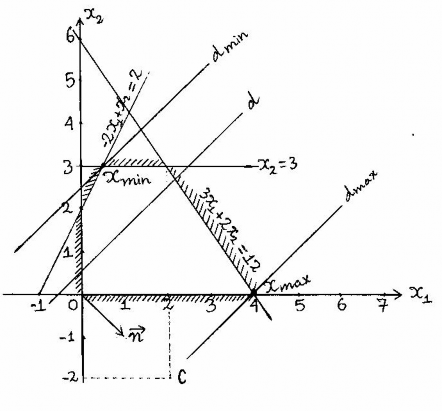
Example 1Solve the following QHTT problem using geometric method. f(x) = 2 x 1-2x 2min ( max)

D:



 3x 1  2x 2  12

- 2x 1 x 2 2

  x 10 , x 20,

x 2 3

Prize



The solution domain D, level curve (d), point C and vector n are determined as shown in the figure.





 Case f min: Translate (d) in the opposite direction to get x m in = ( 1;3) , f m in = -5.

2

n we get d m in and from

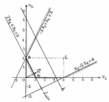
Example 2Solve the following QHTT problem using geometric methods.

f(x) = 4x 1 +2x 2 min ( max)

 2x 1  x 2  2

 x 1  2x 2  4

D:  - 2x 1 x 2 2



 x 10 , x 20

Prize



The solution domain D, level curve (d), point C and vector n are determined as shown in the figure.

 Case f min : Translate (d) in the opposite direction to



n we get d m in and from

that calculates x m in = ( t ; 2-2t) with 0 t 1, f m in = 4. That is, PATU corresponds to the case f min is the whole line segment AB.

 Case f max: Translation (d) in the direction



n we see (d) and D have no points

tangent. That is, the objective function is not bounded above and the problem has no optimal solution.

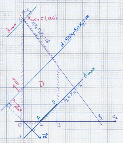
Example 3Solve the following QHTT problem using geometric method. f(x) = 50x 1- 50x 2min (max)

D:



 4x 1  3 x 2  18

 - x 1 x 2  1

  x 1 0 , x 2 0,



x 1  2

Prize



Solution domain D, vector n  (1;  1) OC  (50;  50) , level line ( d ) as shown.



Case f min : Translate (d) in the opposite direction of n to get d m in and

from which we can calculate X min  (0;6) , f min  f (0,6)   300 .

Case f max : Translation (d) in the direction

